<![CDATA[Shady Minds]]>2022-07-25T20:53:02-07:00http://dyagilev.org/Octopress<![CDATA[Building SQL driver for in-memory datagrid. Slides]]>2018-02-02T17:57:37+03:00http://dyagilev.org/blog/2018/02/02/how-we-built-sql-driver-for-in-memory-datagrid-slidesWhat it takes to build a SQL driver for distributed data storage with Apache Calcite. Sharing my experience in the deck.
]]><![CDATA[How we built InsightEdge. Slides and talk recording]]>2017-12-06T12:36:00-08:00http://dyagilev.org/blog/2017/12/06/how-we-built-insightedgeSharing my slides and talk recording (in Russian) from JavaDay 2016 conference.
In this talk I discuss how we built an open-source Spark distribution http://insightedge.io that runs on top of in-memory database.
The agenda of the talk:
a need of hybrid transactional and analytical processing
an overview of in-memory datagrid features
how we designed InsightEdge RDD partitions to make it scalable
implementation of Spark DataSource API to support DataFrame/SQL
optimization techniques: predicates push-down and columns pruning
how InsightEdge can run 30 times faster that regular Spark
designing API with Scala, the good and unpleasant parts
extending Spark API with geo spatial queries
testing with Docker
Video recording (in Russian):
Slides:
]]><![CDATA[Real-time Spatial Analytics with InsightEdge Spark: Taxi Price Surge Use Case]]>2016-09-29T16:35:41+03:00http://dyagilev.org/blog/2016/09/29/real-time-spatial-analytics-with-insightedge-spark-taxi-price-surge-use-caseA couple of weeks ago we launched InsightEdge, introducing you to our high performance Spark distribution with enterprise-grade OLTP capabilities. In this blog post, we will create a demo application for a taxi price surge use case that runs real-time analytics on a streaming geospatial data.
We take a fundamental supply and demand economic model of price determination in a market. We will then compute price in real-time based on the current supply and demand.
To make our demo even more fun, we will create a taxi price surge use case. We will consider the transportation business domain, and taxi companies like Uber or Lyft in particular.
In taxi services, the order requests and available drivers represent the supply and demand data correspondingly. It is interesting that this data is bound to geographical location, which introduces additional complexity. Comparing to business areas like retail, where the product demand is linked to either offline store or a well known list of warehouses, the order requests are geographically distributed.
With services like Uber, the fare rates automatically increase when the taxi demand is higher than drivers around you. The Uber prices are surging to ensure reliability and availability for those who agree to pay a bit more.
Taxi Price Surge Use Case – 3 Key Architectural Questions
How do we handle the events like an ‘Order Request’ event or a ‘Pickup’ event?
How do we compute the price accounting the nearby requests? We will need to find an efficient way to execute geospatial queries.
How can we scale technology to run business in many cities, states or countries?
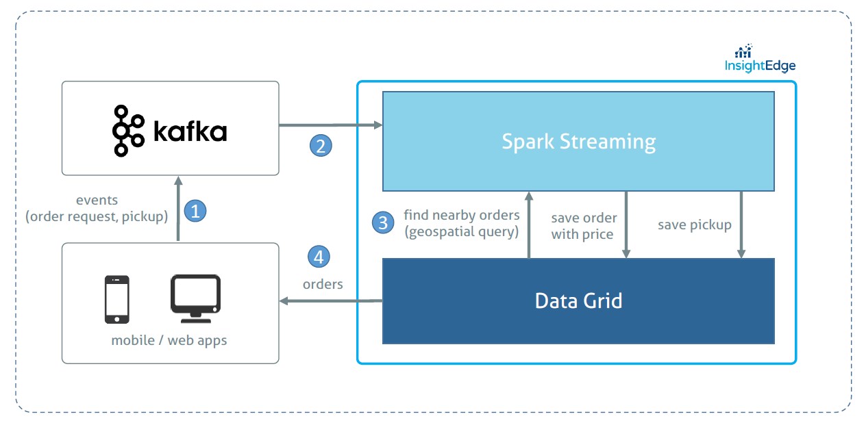
Architecture
The following diagram illustrates the application architecture:
How Does this Architecture Addresses Our 3 Key Questions?
With InsightEdge Geospatial API we are able to efficiently find nearby orders and, therefore, minimize the time required to compute the price. The efficiency comes from the ability to index order request location in the datagrid.
Kafka allows to handle a high throughput of incoming raw events. Even if the computation layer starts processing slower(say during the peak hour), all the events will be reliably buffered in Kafka. The seamless and proven integration with Spark makes it a good choice for streaming applications.
InsightEdge Data Grid also plays a role of a serving layer handling any operational/transactional queries from web/mobile apps.
All the components(Kafka and InsightEdge) can scale out almost linearly;
To scale to many cities, we can leverage data locality principle through a full pipeline (Kafka, Spark, Data Grid) partitioning by the city or even with a more granular geographical units of scale. In this case the geospatial search query will be limited to a single Data Grid partition. We leave this enhancement out of the scope of the demo.
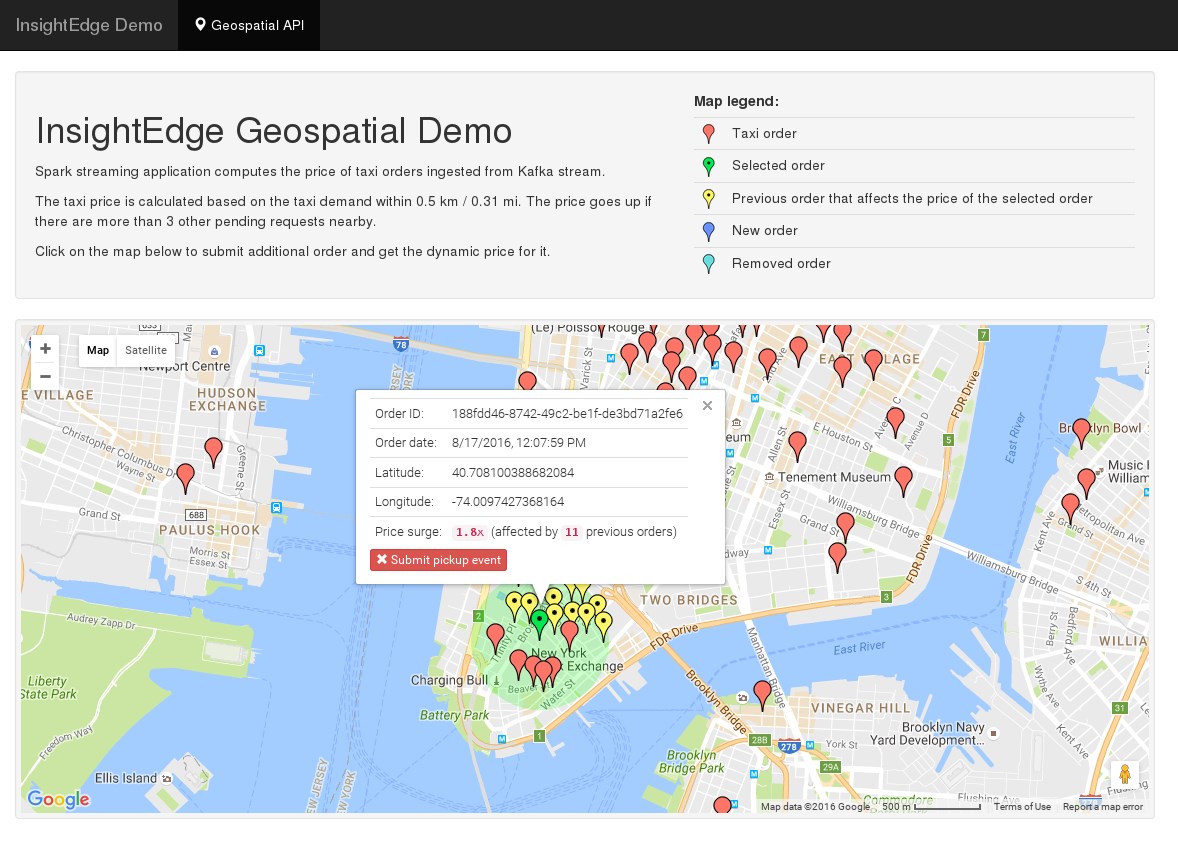
Building a Demo Application for a Taxi Price Surge Use Case
To simulate the taxi orders we took a csv dataset with Uber pickups in New York City. The demo application consists of following components:
Feeder application, reads the csv file and sends order and pickup events to Kafka
InsightEdge processing, a Spark Streaming application that reads from Kafka, computes price and saves to datagrid
Web app, reads orders from datagrid and visualizes them on a map
Coding Processing Logic with InsightEdge API
Let’s see how InsightEdge API can be used to calculate the price:
12345678910111213141516171819202122
valordersStream=initKafkaStream(ssc,"orders")// step 1ordersStream.map(message=>Json.parse(message).as[OrderEvent])// step 2.transform{rdd=>// step 3valquery="location spatial:within ? AND status = ?"valradius=0.5*DistanceUtils.KM_TO_DEGvalqueryParamsConstructor=(e:OrderEvent)=>Seq(circle(point(e.longitude,e.latitude),radius),NewOrder)valprojections=Some(Seq("id"))rdd.zipWithGridSql[OrderRequest](query,queryParamsConstructor,projections)}.map{case(e:OrderEvent,nearOrders:Seq[OrderRequest])=>// step 4vallocation=point(e.longitude,e.latitude)valnearOrderIds=nearOrders.map(_.id)valpriceFactor=if(nearOrderIds.length>3){1.0+(nearOrderIds.length-3)*0.1}else{1.0}OrderRequest(e.id,e.time,location,priceFactor,nearOrderIds,NewOrder)}.saveToGrid()// step 5
Step 1: Initialize a stream of Kafka orders topic
Step 2: Parse Kafka message that is in Json format (in real app you may want to use formats like Avro)
Step 3: For every order we find other non-processed orders within 0.3 km using InsightEdge’s zipWithGridSql() function
Step 4: Given near orders, we calculate the price with a simple linear function
Step 5: Finally we save the order details including price and near order ids into the data grid with saveToGrid()function
The full source of the application is available on github
Taxi Price Surge Use Case Summary
In this blog post we created a demo application that processes the data stream using InsightEdge geospatial features.
An alternative approach for implementing dynamic price surging can use machine learning clustering algorithms to split order requests into clusters and calculate if the demand within a cluster is higher than the supply. This streaming application saves the cluster details in the datagrid. Then, to determine the price we execute a geospatial datagrid query to find which cluster the given location belongs to.
]]><![CDATA[Scalable machine learning with InsightEdge: mobile advertisement clicks prediction]]>2016-05-30T20:34:42+03:00http://dyagilev.org/blog/2016/05/30/scalable-machine-learning-with-insightedge-mobile-advertisement-clicks-predictionThis blog post will provide an introduction into using machine learning algorithms with InsightEdge. We will go through an exercise to predict mobile advertisement click-through rate with Avazu’s dataset.
There are several compensation models in online advertising industry, probably the most notable is CPC (Cost Per Click), in which an advertiser pays a publisher when the ad is clicked.
Search engine advertising is one of the most popular forms of CPC. It allows advertisers to bid for ad placement in a search engine’s sponsored links when someone searches on a keyword that is related to their business offering.
For the search engines like Google, advertising is one of the main sources of their revenue. The challenge for the advertising system is to determine what ad should be displayed for each query that the search engine receives.
The revenue search engine can get is essentially:
revenue = bid * probability_of_click
The goal is to maximize the revenue for every search engine query. Whereis the bid is a known value, the probability_of_click is not. Thus predicting the probability of click becomes the key task.
Working on a machine learning problem involves a lot of experiments with feature selection, feature transformation, training different models and tuning parameters.While there are a few excellent machine learning libraries for Python and R, like scikit-learn, their capabilities are typically limited to relatively small datasets that you fit on a single machine.
With the large datasets and/or CPU intensive workloads you may want to scale out beyond a single machine. This is one of the key benefits of InsightEdge, since it’s able to scale the computation and data storage layers across many machines under one unified cluster.
train (5.9G) - Training set. 10 days of click-through data, ordered chronologically. Non-clicks and clicks are subsampled according to different strategies.
test (674M) - Test set. 1 day of ads to test model predictions.
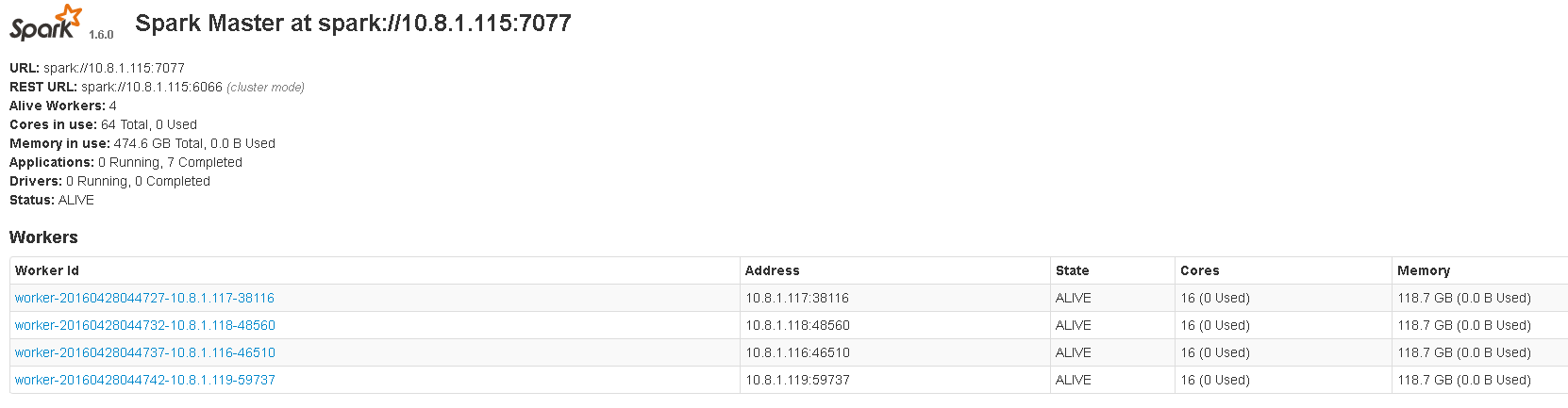
At first, we want to launch InsightEdge.
To get the first data insights quickly, one can launch InsightEdge on a laptop.
Though for the big datasets or compute-intensive tasks the resources of a single machine might not be enough.
For this problem we will setup a cluster with four workers and place the downloaded files on HDFS.
Let’s open the interactive Web Notebook and start exploring our dataset.
The dataset is in csv format, so we will use databricks csv library to load it from hdfs into the Spark dataframe:
Let’s see how many rows are in the training dataset:
123
valtotalCount=df.count()totalCount:Long=40428967
There are about 40M+ rows in the dataset.
Let’s now calculate the CTR (click-through rate) of the dataset. The click-through rate is the number of times a click is made on the advertisement divided by the total impressions (the number of times an advertisement was served):
The CTR is 0.169 (or 16.9%) which is quite a high number, the common value in the industry is about 0.2-0.3%. So a high value is probably because non-clicks and clicks are subsampled according to different strategies, as stated by Avazu.
Now, the question is which features should we use to create a predictive model? This is a difficult question that requires a deep knowledge of the problem domain. Let’s try to learn it from the dataset we have.
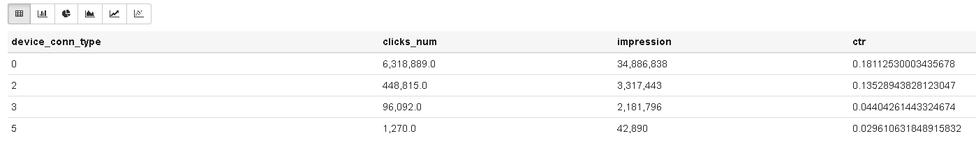
For example, let’s explore the device_conn_type feature. Our assumption might be that this is a categorical variable like Wi-Fi, 2G, 3G or LTE. This might be a relevant feature since clicking on an ad with a slow connection is not something common.
At first, we register the dataframe as a SQL table:
We see that there are four connection type categories. Two categories with CTR 18% and 13%, and the first one is almost 90% of the whole dataset. The other two categories have significantly lower CTR.
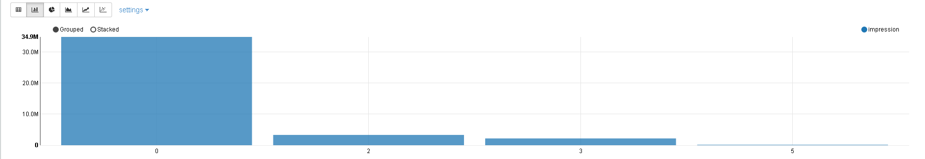
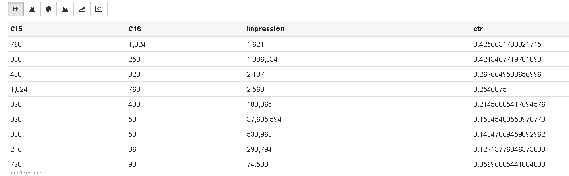
Another observation we may notice is that features C15 and C16 look like the ad size:
We can notice some correlation between the ad size and its performance. The most common one appears to be 320x50px known as “mobile leaderboard” in Google AdSense.
What about other features? All of them represent categorical values, how many unique categories for each feature?
We see that there are some features with a lot of unique values, for example, device_ip has 6M+ different values.
Machine learning algorithms are typically defined in terms of numerical vectors rather than categorical values. Converting such categorical features will result in a high dimensional vector which might be very expensive.
We will need to deal with this later.
Processing and transforming the data
Looking further at the dataset, we can see that the hour feature is in YYMMDDHH format.
To allow the predictive model to effectively learn from this feature it makes sense to transform it into three features: year, month and hour.
Let’s develop the function to transform the dataframe:
The entire training dataset contains 40M+ rows, it takes quite a long time to experiment with different algorithms and approaches even in a clustered environment.
We want to sample the dataset and checkpoint it to the in-memory data grid that is running collocated with Spark.
This way we can:
* quickly iterate through different approaches
* restart the Zeppelin session or launch other Spark applications and pick up the dataset more quickly from memory
Since the training dataset contains the data for the 10 days, we can pick any day and sample it:
The complete listing of notebook can be found on github. You can import it to Zeppelin and play with it on your own.
A simple algorithm
Now that we have training and test datasets sampled, initially preprocessed and available in the data grid, we can close Web Notebook and start experimenting with
different techniques and algorithms by submitting Spark applications.
For our first baseline approach let’s take a single feature device_conn_type and logistic regression algorithm:
importcom.gigaspaces.spark.context.GigaSpacesConfigimportcom.gigaspaces.spark.implicits._importorg.apache.spark.ml.feature.{OneHotEncoder,StringIndexer}importorg.apache.spark.mllib.classification.LogisticRegressionWithLBFGSimportorg.apache.spark.mllib.evaluation.BinaryClassificationMetricsimportorg.apache.spark.mllib.linalg.Vectorimportorg.apache.spark.mllib.regression.LabeledPointimportorg.apache.spark.sql.SQLContextimportorg.apache.spark.sql.insightedge._importorg.apache.spark.{SparkConf,SparkContext}objectCtrDemo1{defmain(args:Array[String]):Unit={if(args.length<3){System.err.println("Usage: CtrDemo1 <spark master url> <grid locator> <train collection>")System.exit(1)}valArray(master,gridLocator,trainCollection)=args// Configure InsightEdge settingsvalgsConfig=GigaSpacesConfig("insightedge-space",None,Some(gridLocator))valsc=newSparkContext(newSparkConf().setAppName("CtrDemo1").setMaster(master).setGigaSpaceConfig(gsConfig))valsqlContext=newSQLContext(sc)// load training collection from data gridvaltrainDf=sqlContext.read.grid.load(trainCollection)trainDf.cache()// use one-hot-encoder to convert 'device_conn_type' categorical feature into a vectorvalindexed=newStringIndexer().setInputCol("device_conn_type").setOutputCol("device_conn_type_index").fit(trainDf).transform(trainDf)valencodedDf=newOneHotEncoder().setDropLast(false).setInputCol("device_conn_type_index").setOutputCol("device_conn_type_vector").transform(indexed)// convert dataframe to a label points RDDvalencodedRdd=encodedDf.map{row=>vallabel=row.getAs[Double]("click")valfeatures=row.getAs[Vector]("device_conn_type_vector")LabeledPoint(label,features)}// Split data into training (60%) and test (40%)valArray(trainingRdd,testRdd)=encodedRdd.randomSplit(Array(0.6,0.4),seed=11L)trainingRdd.cache()// Run training algorithm to build the modelvalmodel=newLogisticRegressionWithLBFGS().setNumClasses(2).run(trainingRdd)// Clear the prediction threshold so the model will return probabilitiesmodel.clearThreshold// Compute raw scores on the test setvalpredictionAndLabels=testRdd.map{caseLabeledPoint(label,features)=>valprediction=model.predict(features)(prediction,label)}// Instantiate metrics objectvalmetrics=newBinaryClassificationMetrics(predictionAndLabels)valauROC=metrics.areaUnderROCprintln("Area under ROC = "+auROC)}}
We will explain a little bit more what happens here.
At first, we load the training dataset from the data grid, which we prepared and saved earlier with Web Notebook.
Then we use StringIndexer and OneHotEncoder to map a column of categories to a column of binary vectors. For example, with 4 categories of device_conn_type, an input value
of the second category would map to an output vector of [0.0, 1.0, 0.0, 0.0, 0.0].
Then we convert a dataframe to an RDD[LabeledPoint] since the LogisticRegressionWithLBFGS expects RDD as a training parameter.
We train the logistic regression and use it to predict the click for the test dataset. Finally we compute the metrics of our classifier comparing the predicted labels with actual ones.
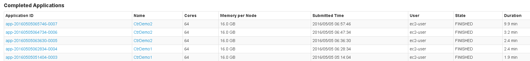
To build this application and submit it to the InsightEdge cluster:
It takes about 2 minutes for the application to complete and output the following:
1
Area under ROC= 0.5177127622153417
We get AUROC slightly better than a random guess (AUROC = 0.5), which is not so bad for our first approach, but we can definitely do better.
Experimenting with more features
Let’s try to select more features and see how it affects our metrics.
For this we created a new version of our app CtrDemo2 where we
can easily select features we want to include. We use VectorAssembler to assemble multiple feature vectors into a single features one:
You can notice how the AUROC is being improved as we add more and more features. This comes with the cost of the training time:
We didn’t include high-cardinality features such as device_ip and device_id as they will blow up the feature vector size. One may consider applying techniques such as feature hashing
to reduce the dimension. We will leave it out of this blog post’s scope.
Tuning algorithm parameters
Tuning algorithm parameters is a search problem. We will use Spark Pipeline API with a Grid Search technique.
Grid search evaluates a model for each combination of algorithm parameters specified in a grid (do not confuse with data grid).
Pipeline API supports model selection using cross-validation technique. For each set of parameters it trains the given Estimator and evaluates it using the given Evaluator.
We will use BinaryClassificationEvaluator that has AUROC as a metric by default.
We included two regularization parameters 0.01 and 0.1 in our search grid for now, others are commented out for now.
Output the best set of parameters:
1234567
println("Grid search results:")cvModel.getEstimatorParamMaps.zip(cvModel.avgMetrics).foreach(println)println("Best set of parameters found:"+cvModel.getEstimatorParamMaps.zip(cvModel.avgMetrics).maxBy(_._2)._1)
Use the best model to predict test dataset loaded from the data grid:
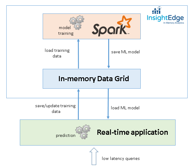
The following diagram demonstrates the design of machine learning application with InsightEdge.
The key design advantages are:
the single platform converges analytical processing (machine learning) powered by Spark with transactional processing powered by custom real-time applications;
real-time applications can execute any OLTP query (read, insert, update, delete) on training data that is immediately available for Spark analytical queries or machine learning routines. There is no need to build a complex ETL pipeline that extracts training data from OLTP database with Kafka/Flume/HDFS. Besides the complexity, an ETL pipeline introduces unwanted latency that can be a stopper for reactive machine learning apps.
With InsightEdge, Spark applications can view the live data;
the training data lives in the memory of data grid, which acts as an extension of Spark memory. This way we can load the data quicker;
An in-memory data grid is a general-purpose highly available and fault tolerant storage. With support of ACID transactions and SQL queries it becomes the primary storage for the application;
InsightEdge stack is scalable in both computation (Spark) and storage (data grid) tiers. This makes it attractive for large-scale machine learning.
Summary
In this blog post we demonstrated how to use machine learning algorithms with InsightEdge. We went through typical stages:
interactive data exploration with Zeppelin
feature selection and transformation
training predictive models
calculating model metrics
tuning parameters
We didn’t have a goal to build a perfect predictive model, so there is great room for improvement.
In the architecture section we discussed how the typical design may look like, what are the benefits of using InsightEdge for machine learning.
The Zeppelin notebook can be found here and submittable spark apps here
]]><![CDATA[Java enums in distributed systems]]>2016-01-20T23:01:20+02:00http://dyagilev.org/blog/2016/01/20/java-enums-in-distributed-systemsDid you ever think about how hashCode() of java.lang.Enum implemented?
Surprisingly or not it’s
123
publicfinalinthashCode(){returnsuper.hashCode();}
it returns the Object’s hashCode which is an internal address of the object to a certain extend. From the first glance it totally makes sense since Enum values are singletons.
Now imagine you are building distributed system. Distributed systems use hashCode to
determine which worker in a cluster should handle part of a huge job
determine which node in a cluster should store given item of dataset (e.g. in distributed cache)
The same Enum instance would give you a different hashCode value in different JVMs/hosts, screwing up your Hadoop job or put/lookup in distributed storage. Just something I faced recently.
]]><![CDATA[Slides for my JavaDay 2015 talk]]>2015-10-03T20:03:35+03:00http://dyagilev.org/blog/2015/10/03/slides-for-my-javaday-2015-talkSlides for my JavaDay 2015 talk …
]]><![CDATA[Resilient distributed systems with Netflix Hystrix]]>2015-08-10T20:20:31+03:00http://dyagilev.org/blog/2015/08/10/resilient-distributed-systems-with-netflix-hystrixSlides of my talk on building resilient systems with Hystrix …
]]><![CDATA[Understanding Parser Combinators in Scala]]>2015-07-15T21:50:16+03:00http://dyagilev.org/blog/2015/07/15/understanding-parser-combinators-in-scalaSlides of my talk on Parser Combinators in internal Scala School …
We will gradually build an embedded domain-specific language (DSL) for specifying grammars in a EBNF-like notation in Scala.
We will use monadic parser combinators approach. As a result we should be able to parse JSON document using our library.
]]><![CDATA[Distributed Configuration for SaaS application]]>2015-06-01T21:36:36+03:00http://dyagilev.org/blog/2015/06/01/distributed-configuration-for-saas-applicationRecently I was involved into discussion of SaaS application design. One of the questions was how to manage configuration in large scale SaaS. The rise of clouds, microservices and container virtualization influence approaches used in configuration management. In this article we will look what we can learn from these concepts and how we can apply these lessons in SaaS and other generic distributed systems. In the second part of the article, we will build a PoC of elastic tenant aware application leveraging Zookeeper with 200 lines in Scala.
Before considering any architecture, let’s refresh what requirements are essential for typical SaaS application:
elasticity, ability to add and remove tenants in runtime with zero system downtime
scalability, ability to handle growing amount of users
availability, the service should stay functional and usable to fulfil business requirements
(we skip other fundamental requirements such as security as they are not primary focus of the article)
Okay, how do we usually deal with scalability concerns?
When it comes to application services(or application servers), we prefer making them stateless, so we can simply run multiple copies and distribute load between them achieving scaling out (horizontal) capabilities. And what about availability? Pretty the same, run redundant copies of your service. So far so good.
Okay, but having hundreds of customers(tenants) multiplied on number of application servers per customer requires unreasonable overhead on memory, CPU and other hardware resources. Usually customers are different in size, usage patterns and timezones. Under these conditions generated load is spread unequally and lead to suboptimal resources utilization. Further cost overhead comes from licenses of underlying software(databases, application servers, operating systems, etc).
Multitenancy comes to the rescue. Multitenancy implies the ability to serve multiple tenants with a single application instance thus spreading the load more equally and amortizing infrastructure overhead. Though multitenancy is not free, the downside is the increased engineering complexity that requires additional development effort. On the other hand some of these issues can be partially addressed with virtualization, it looks attractive since doesn’t require any significant architecture redesign.
Having scalable application server layer is only part of the problem, with growing amount of customers the data storage has to be scalable as well. Designing multitenant data storage is another huge topic, we will not dig into consideration details. While NoSQL solutions are able to scale out of the box, with relational databases we have to scale them manually allocating database instance per one or several customers, thus application server instance may talk to multiple databases.
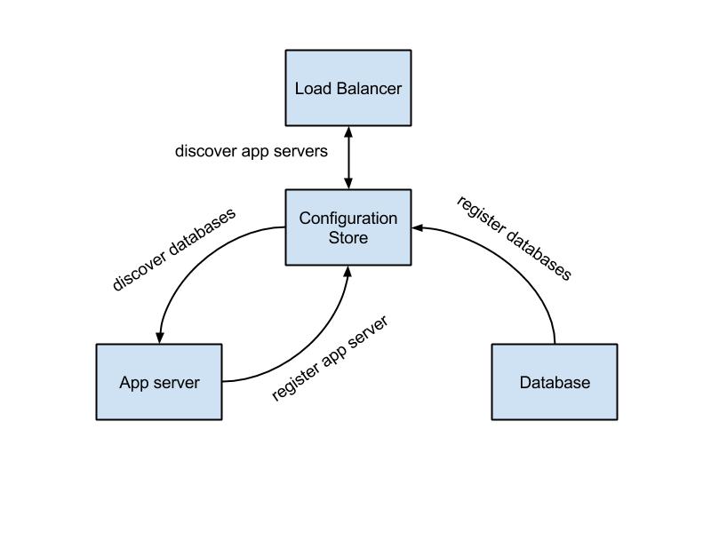
Remember, in dynamic scalable SaaS environment application servers, databases and load balancer instances come and go while relying on each other combining a distributed cluster. The load balancer should know about application server instances, and application server instance should talk to databases. So when the database for new customer is provisioned, some or all application servers have to be notified about database layer changes and load balancer has to be notified of all changes in a farm of application servers. In short, we need an ability to link the pieces of multi-tier application together in realtime.
Configuration management tools like Chef, Puppet, etc are able to configure a node based on centralized configuration, though they are not designed to be responsive and propagate configuration changes quickly. Additionally they are not designed to detect failures or tolerate network partitions.
If you think about multi-tier configuration in a more abstract way, you will easily recognize service registry and service discovery patterns that people use many years building distributed systems.
Even more, with the rise of container based virtualization and Docker in particularly, service discovery becomes very important part. Containers need an ability to discovery each other adopting to the current environment.
Let’s see how SaaS configuration will look from service discovery perspective.
Okay, but can we just use simple database with inserts and selects to register and discovery? Well, there are a few concerns with that:
availability, configuration store should be distributed and tolerate nodes failure, otherwise it will be a single point of failure.
service failure detection, we need some sort of services monitoring, if service goes down, dependent services should react correspondingly. The are several approaches for failure detection design. Client can keep TCP connection indicating it’s alive, service can periodically send messages or configuration store itself can monitor service endpoint. This design decision is a subject for debates, one should consider what is reasonable in the context. There a few available service discovery tools following these patterns.
Now that we have discussed the high level design and requirements of configuration store, we can briefly mention open source tools: Zookeeper, Consul, etcd, Eureka, SmartStack, Doozer, Serf, etc.
I would highlight three of them definitely worth checking:
Apache Zookeeper. Written in Java, choses consistency over availability, old, mature, battle-tested, very popular in middleware(Hadoop, Kafka, Storm, etc). Hard to use properly because of low level API. Consider using existing recipes or Curator library.
HashiCorp Consul. Written in Go, flexible between consistency and availability, new and promising, high level features out of the box, multi datacenter support.
Airbnb SmartStack. Written in Ruby on top of Zookeeper and HAProxy, unique design where application service talks to HAProxy on localhost, adds Zookeeper caching to favour availability over consistency.
Part 2. Building a PoC
Let’s build a simple demo application to proof the concept described above. We will try to simplify things as much as possible sacrificing correctness and errors handling sometimes, but still suitable for illustration purpose. Note, one should leverage existing Curator service discovery recipes when building production quality applications. The source code is available on github
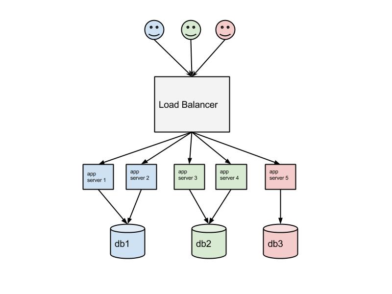
For this PoC we choose tenant aware model rather than multitenancy to demonstrate how to incorporate custom logic with service discovery. In this model client (tenant) is routed to a configurable number of application services while they use common database.
Beware that this model has its drawbacks such as weaker scale-in (reducing the quantity of servers) and cost saving capabilities since the load is not equally spread comparing to true multitenancy. On the other hand this can be compensated with container virtualization in some sort. Also this model implies support of multiple release versions of application and has better support of application level caching. Again, the tenancy model itself is not a subject here rather than a centralized configuration.
Spray(runs on top of Akka) for lightweight http services
HAProxy load balancer
Zookeeper data model
We define Zookeeper data model as a following hierarchical structure.
/app
  /client-{id}
    /db
    /app-server-slots
Znode /db contains database details such as connection url. Znode /app-server-slots defines the maximum number of application server instances we want to run for given client.
Here is an example with 3 clients, the value of znode follows = sign.
Service registration is implemented using so called ephemeral znodes. Unlike standard znodes they exist as long as the session that created the znode is active.
When application server starts it registers itself creating ephemeral znode under corresponding client. Respectively when application server is brought down or it failures for some reason, the ephemeral znode is automatically deleted. The value of znode contains http service location.
We use HAProxy as a load balancer. To reconfigure HAProxy in runtime we created a simple agent that runs alongside HAProxy process and watches for any configuration changes. Once it detects any changes in Zookeeper, it rewrites HAProxy config and send a command to reload it.
How it works in action
At first we start Zookeeper zkServer.sh start
Then we create some data model to play with by running ZkSchemaBuilder.scala. You can browse zookeeper data with zkCli.sh tool.
Start HAProxy /haproxy/start.sh and HAProxy agent running HAProxyAgent.scala
At this point we should be able to hit http://localhost:8080/ though it will return 503 since there are no actual backend services running. Let’s fix it.
Run Boot.scala to start application server with http service.
[INFO] [06/01/2015 20:22:16.084] [on-spray-can-akka.actor.default-dispatcher-2] [akka://on-spray-can/user/IO-HTTP/listener-0] Bound to Oleksiis-Mac-mini.local/192.168.0.100:57581
registering service available at Oleksiis-Mac-mini.local:57581
looking for a client with free slots
client client-1 slots: 2 occupied: 0
Found client client-1 with available slot(s) ... registering
Configuring HttpService with dbUrl jdbc://db-client-1:5555
We see that http service was brought up for client-1 that had 2 available slots.
Now run Boot.scala several more times to start more servers and check haproxy/haproxy.conf
defaults
 mode http
 timeout connect 5000ms
 timeout client 50000ms
 timeout server 50000ms

frontend http-in
 bind *:8080
 acl client-1-path path_beg /client-1
 acl client-2-path path_beg /client-2
 acl client-3-path path_beg /client-3
 use_backend client-1-backend if client-1-path
 use_backend client-2-backend if client-2-path
 use_backend client-3-backend if client-3-path

backend client-1-backend
 balance roundrobin
 server app Oleksiis-Mac-mini.local:57581
 server app Oleksiis-Mac-mini.local:57588

backend client-2-backend
 balance roundrobin
 server app Oleksiis-Mac-mini.local:57591
 server app Oleksiis-Mac-mini.local:57595

backend client-3-backend
 balance roundrobin
 server app Oleksiis-Mac-mini.local:57598
As we see HAProxy agent observed and propagated all configuration changes to haproxy.conf. We use HAProxy acl feature to route http requests by url prefix, i.e. requests starting with /client-1 will be routed to a farm of application servers serving for client-1.
Now if we hit http://localhost:8080/client-1/test we should get a response “OK. Http service configured with db url: jdbc://db-client-1:5555”. Voila!
You should also notice that killing an application server process will result in immediate reconfiguration of HAProxy.
]]><![CDATA[Spring Data and type-safe API for GigaSpaces XAP]]>2015-04-12T21:21:13+03:00http://dyagilev.org/blog/2015/04/12/spring-data-and-type-safe-api-for-gigaspaces-xapWe have developed Spring Data API for GigaSpaces XAP with a number of fancy extensions. Check it out on github
Motivation:
make it easy to use in-memory datagrid for those who already have experience with Spring Data APIs such as Spring Data MongoDB, JPA, Redis, etc.
significantly reduce the amount of boilerplate code required to implement data access layer
reduce the amount of effort in switching from any Spring Data implementation to XAP
catch API errors at compile time (type-safe API using QueryDSL)
Features
Spring configuration support using Java based @Configuration classes or XML namespace, filters support
CRUD and Paging repositories extended with XAP specific features such as projections, change API, lease, take, etc
repository for XAP Documents
selectively exposing CRUD methods
query methods (e.g. findByNameAndAge)
custom methods
common query lookup strategies
property expressions
special parameters handling including Sort and Pageable
native XAP API support
seamless integration with all native XAP features - persistence, transcations, event processing, security, indexes, lease, etc
ability to work with multiple spaces
QueryDSL integration to support type-safe API(queries, projection, change API)
]]><![CDATA[Keep up with Spark Streaming at in-memory speed using GigaSpaces XAP]]>2015-03-07T21:33:06+02:00http://dyagilev.org/blog/2015/03/07/Keep-up-with-Spark-Streaming-at-in-memory-speed-using-GigaSpaces-XAPSpark Streaming is a popular engine for stream processing and its ability to compute data in memory makes it very attractive. However Spark Streaming is not self-sufficient, it relies on external data source and storage to output computation results. Therefore, in many cases the overall performance is limited by slow external components that are not able to keep up with Spark’s throughput and/or introduce unacceptable latency.
In this article we describe how we use GigaSpaces XAP in-memory datagrid to address this challenge. Code sources are available on github
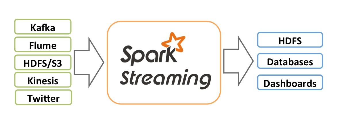
Real-time processing is becoming more and more popular. Spark Streaming is an extension of the core Spark API that allows scalable, high-throughput, fault-tolerant stream processing of live data streams.
Spark Streaming has many use cases: user activity analytics on web, recommendation systems, censor data analytics, fraud detection, sentiment analytics and more.
Data can be ingested to Spark cluster from many sources like HDS, Kafka, Flume, etc and can be processed using complex algorithms expressed with high-level functions like map, reduce, join and window. Finally, processed data can be pushed out to filesystems or databases.
Challenge
Spark cluster keeps intermediate chunks of data (RDD) in memory and, if required, rarely touches HDFS to checkpoint stateful computation, therefore it is able to process huge volumes of data at in-memory speed. However, in many cases the overall performance is limited by slow input and output data sources that are not able to stream and store data with in-memory speed.
Solution
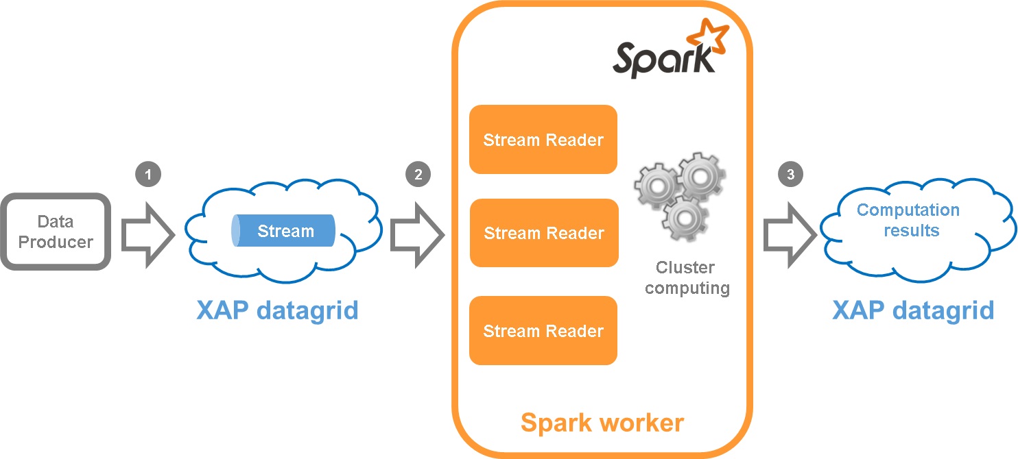
In this pattern we address performance challenge by integrating Spark Streaming with XAP. XAP is used as a stream data source and a scalable, fast, reliable persistent storage.
Producer writes the data to XAP stream
Spark worker reads the data from XAP stream and propagates it further for computation
Spark saves computation results to XAP datagrid where they can be queried to display on UI
Let’s discuss this in more details.
XAP Stream
On XAP side we introduce the concept of stream. Please find XAPStream – an implementation that supports writing data in single and batch modes and reading in batch mode. XAPStream leverages XAP’s FIFO (First In, First Out) capabilities.
Here is an example how one can write data to XAPStream. Let’s consider we are building a Word Counter application and would like to write sentences of text to the stream.
At first we create a data model that represents a sentence. Note, that the space class should be annotated with FIFO support.
Complete sources of Sentence.java can be found here
Spark Input DStream
In order to ingest data from XAP to Spark, we implemented a custom ReceiverInputDStream that starts the XAPReceiver on Spark worker nodes to receive the data.
XAPReceiver is a stream consumer that reads batches of data in multiple threads in parallel to achieve the maximum throughput.
XAPInputDStream can be created using the following function in XAPUtils object.
12345678910111213
/** * Creates InputDStream with GigaSpaces XAP used as an external data store * * @param ssc streaming context * @param storageLevel RDD persistence level * @param template template used to match items when reading from XAP stream * @param batchSize number of items to read from * @param readRetryInterval time to wait till the next read attempt if nothing consumed * @param parallelReaders number of parallel readers * @tparam T Class type of the object of this stream * @return Input DStream */defcreateStream[T<:java.io.Serializable:ClassTag](ssc:StreamingContext,template:T,batchSize:Int,readRetryInterval:Duration=Milliseconds(100),parallelReaders:Int,storageLevel:StorageLevel=MEMORY_AND_DISK_SER){…}
Here is an example of creating XAP Input stream. At first we set XAP space url in Spark config:
Output operations allow the DStream’s data to be pushed out to external systems. Please refer to Spark documentation for the details.
To minimize the cost of creating XAP connection for each RDD, we created a connection pool named GigaSpaceFactory. Here is an example how to output RDD to XAP:
Please, note that in this example a XAP connection is created and data is written from Spark driver. In some cases, one may want to write data from the Spark worker. Please, refer to Spark documentation - it explains different design patterns using foreachRDD.
Word Counter Demo
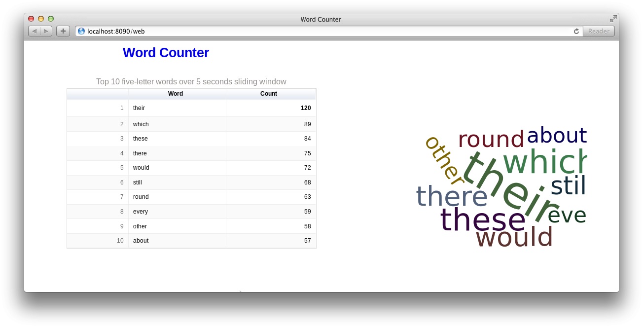
As a part of this integration pattern, we demonstrate how to build an application that consumes live stream of text and displays top 10 five-letter words over a sliding window in real-time. The user interface consists of a simple single page web application displaying a table of top 10 words and a word cloud. The data on UI is updated every second.
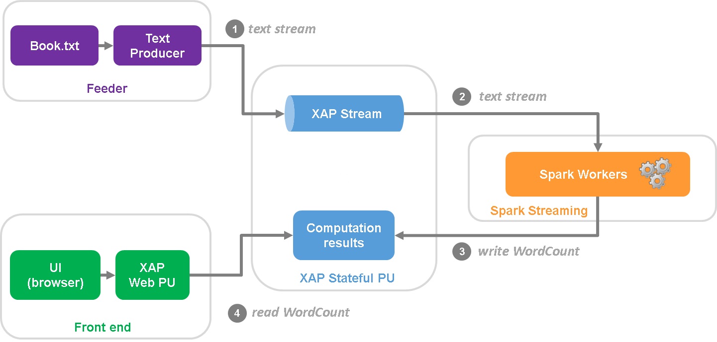
High-level design
The high-level design diagram of the Word Counter Demo is below:
Feeder is a standalone scala application that reads book from text file in a cycle and writes lines to XAP Stream.
Stream is consumed by the Spark cluster which performs all necessary computing.
Computation results are stored in the XAP space.
End user is browsing the web page hosted in a Web PU that continuously updates dashboard with AJAX requests backed by the rest service.
Set the XAP lookup group to spark by adding export LOOKUPGROUPS=spark line to <XAP_HOME>/bin/setenv.sh/bat
Start a Grid Service Agent by running the gs-agent.sh/bat script
Deploy a space by running mvn os:deploy -Dgroups=spark from <project_root>/word-counter-demo directory
Launch Spark Application
Option A. Run embedded Spark cluster
This is the simplest option that doesn’t require downloading and installing Spark distributive, which is useful for the development purposes. Spark runs in the embedded mode with as many worker threads as logical cores on your machine.
Navigate to the <project_root>/word-counter-demo/spark/target directory
Run the following command java -jar spark-wordcounter.jar -s jini://*/*/space?groups=spark -m local[*]
Option B. Run Spark standalone mode cluster
In this option Spark runs a cluster in the standalone mode (as an alternative to running on a Mesos or YARN cluster managers).
Run Spark
Download Spark (tested with Spark 1.2.1 pre-built with Hadoop 2.4)
Follow instructions to run a master and 2 workers. Here is an example of commands with hostname fe2s (remember to substitute it with yours)
Navigate to <project_root>/word-counter-demo/feeder/target
Run java -jar feeder.jar -g spark -n 500
At this point all components should be up and running. The application is available at http://localhost:8090/web/
]]><![CDATA[Slides for my talk on Storm, Kafka and GigaSpaces]]>2014-09-23T18:39:26+03:00http://dyagilev.org/blog/2014/09/23/slides-for-my-talk-on-storm-kafka-gigaspacesCan be found here
]]><![CDATA[GigaSpaces and Storm integration]]>2014-08-21T17:27:50+03:00http://dyagilev.org/blog/2014/08/21/gigaspaces-stormReal-time processing is becoming very popular, and Storm is a popular open source framework and runtime used by Twitter for processing real-time data streams. Storm addresses the complexity of running real time streams through a compute cluster by providing an elegant set of abstractions that make it easier to reason about your problem domain by letting you focus on data flows rather than on implementation details.
Storm has many use cases: realtime analytics, online machine learning, continuous computation, distributed RPC, ETL, and more. Storm is fast: a benchmark clocked it at over a million tuples processed per second per node. It is scalable, fault-tolerant, guarantees your data will be processed, and is easy to set up and operate.
This pattern integrates XAP with Storm. XAP is used as stream data source and fast reliable persistent storage, whereas Storm is in charge of data processing. We support both pure Storm and Trident framework.
As part of this integration we provide classic Word Counter and Twitter Reach implementations on top of XAP and Trident.
Also, we demonstrate how to build highly available, scalable equivalent of Realtime Google Analytics application with XAP and Storm. Application can be deployed to cloud with one click using Cloudify.
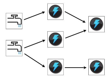
Storm is a real time, open source data streaming framework that functions entirely in memory. It constructs a processing graph that feeds data from an input source through processing nodes. The processing graph is called a “topology”. The input data sources are called “spouts”, and the processing nodes are called “bolts”. The data model consists of tuples. Tuples flow from Spouts to the bolts, which execute user code. Besides simply being locations where data is transformed or accumulated, bolts can also join streams and branch streams.
Storm is designed to be run on several machines to provide parallelism. Storm topologies are deployed in a manner somewhat similar to a webapp or a XAP processing unit; a jar file is presented to a deployer which distributes it around the cluster where it is loaded and executed. A topology runs until it is killed.
Beside Storm, there is a Trident – a high-level abstraction for doing realtime computing on top of Storm. Trident adds primitives like groupBy, filter, merge, aggregation to simplify common computation routines. Trident has consistent, exactly-once semantics, so it is easy to reason about Trident topologies.
Capability to guarantee exactly-once semantics comes with additional cost. To guarantee that, incremental processing should be done on top of persistence data source. Trident has to ensure that all updates are idempotent. Usually that leads to lower throughput and higher latency than similar topology with pure Storm.
Spouts
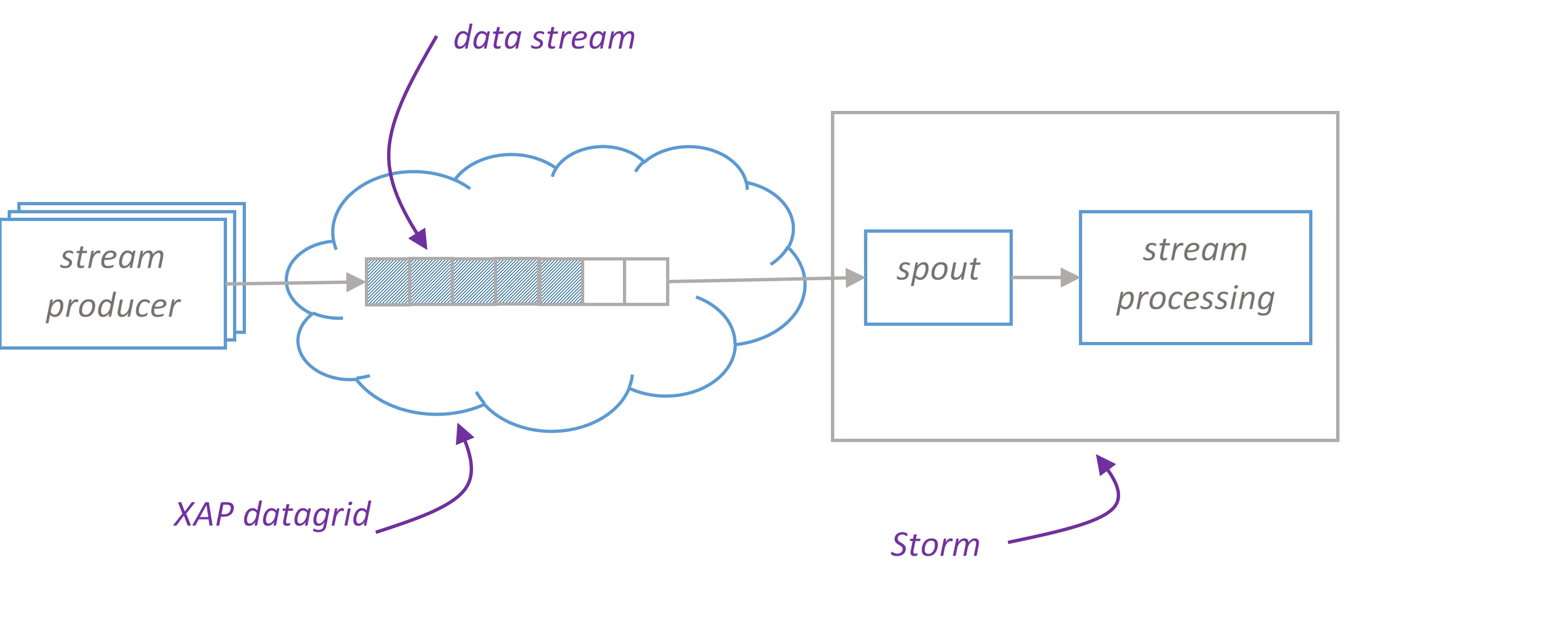
Basically, Spouts provide the source of tuples for Storm processing. For spouts to be maximally performant and reliable, they need to provide tuples in batches, and be able to replay failed batches when necessary. Of course, in order to have batches, you need storage, and to be able to replay batches, you need reliable storage. XAP is about the highest performing, reliable source of data out there, so a spout that serves tuples from XAP is a natural combination.
Depending on domain model and level of guarantees you want to provide, you choose either pure Storm or Trident. We provide Spout implementations for both – XAPSimpleSpout and XAPTranscationalTridentSpout respectively.
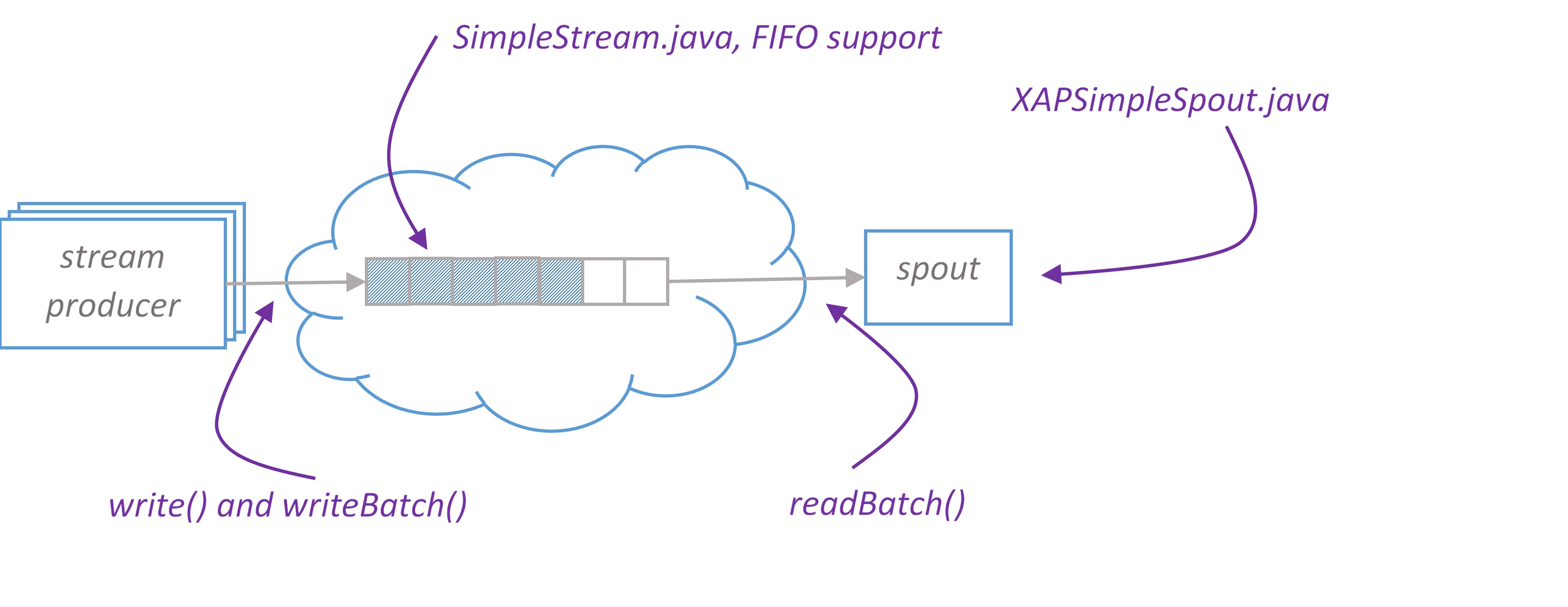
Storm Spout
XAPSimpleSpout is a spout implementation for pure Storm that reads data in batches from XAP. On XAP side we introduce conception of stream. Please find SimpleStream – a stream implementation that supports writing data in single and batch modes and reading in batch mode. SimpleStream leverages XAP’s FIFO(First In, First Out) capabilities.
SimpleStream works with arbitrary space class that has FifoSupport.OPERATION annotation and implements Serializable.
Here is an example how one may write data to SimpleStream and process it in Storm topology. Let’s consider we would like to build an application to analyze the stream of page views (user clicks) on website. At first, we create a data model that represents a page view
The second argument of SimpleStream is a template used to match objects during reading.
If you want to have several streams with the same type, template objects should differentiate your streams.
ConfigConstants. XAP_STREAM_BATCH_SIZE is a maximum number of items that spout reads from XAP with one hit.
Trident Spout
XAPTranscationalTridentSpout is a scalable, fault-tolerant, transactional spout for Trident, supports pipelining. Let’s discuss all its properties in details.
For spout to be maximally performant, we want an ability to scale the number of instances to control the parallelism of reader threads.
There are several spout APIs available that we could potentially use for our XAPTranscationalTridentSpout implementation:
IPartitionedTridentSpout: A transactional spout that reads from a partitioned data source. The problem with this API is that it doesn’t acknowledge when batch is successfully processed which is critical for in memory solutions since we want to remove items from the grid as soon as they have been processed. Another option would be to use XAP’s lease capability to remove items by time out. This might be unsafe, if we keep items too long, we might consume all available memory.
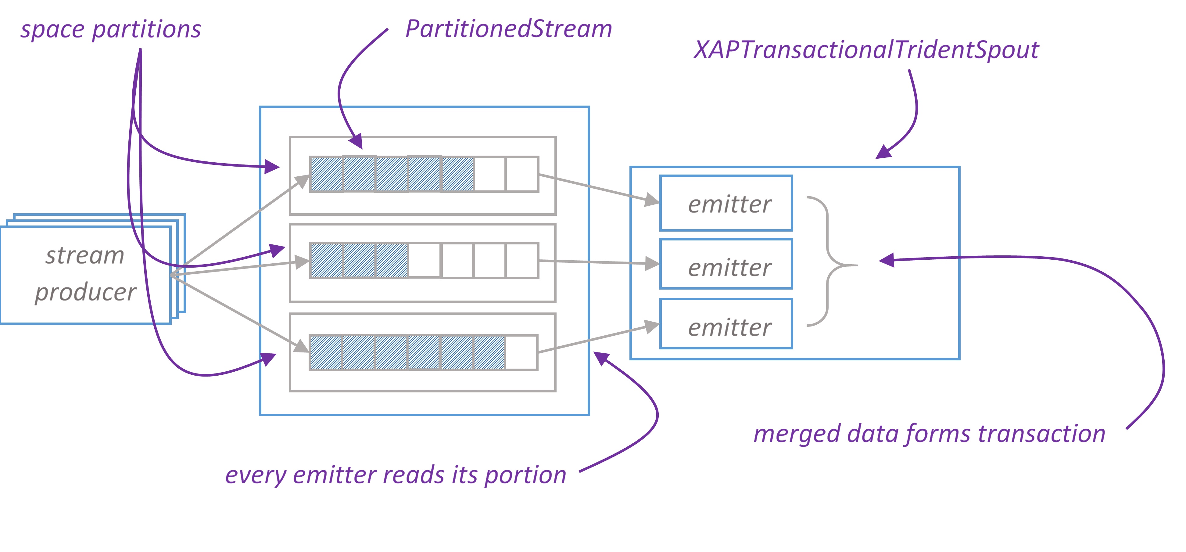
ITridentSpout: The most general API. Setting parallelism hint for this spout to N will create N spout instances, single coordinator and N emitters. When coordinator issues new transaction id, it passes this id to all emitters. Emitter reads its portion of transaction by given transaction id. Merged data from all emitters forms transaction.
For our implementation we choose ITridentSpout API.
There is one to one mapping between XAP partitions and emitters.
Storm framework guarantees that topology is high available, if some component fails, it restarts it. That means our spout implementation should be stateless or able to recover its state after failure.
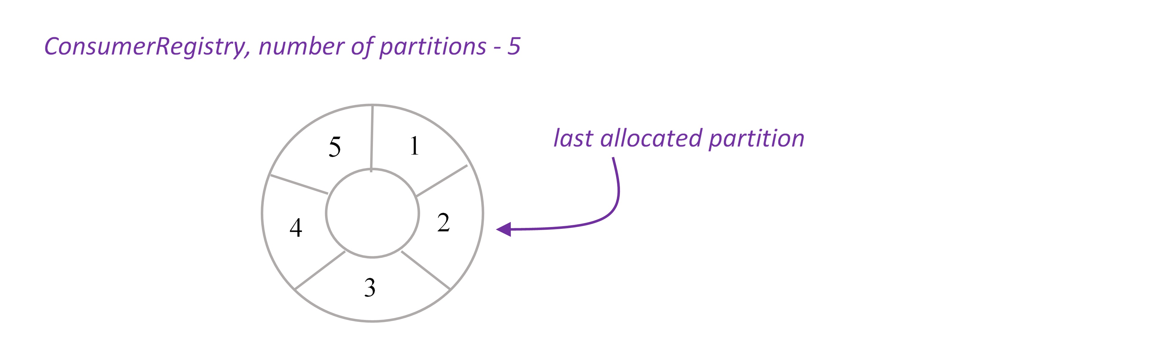
When emitter is created, it calls remote service ConsumerRegistryService to register itself. ConsumerRegistryService knows the number of XAP partitions and keeps track of the last allocated partition. This information is reliably stored in the space, see ConsumerRegistry.java.
Remember that parallelism hint for XAPTranscationalTridentSpout should equal to the number of XAP partitions.
The property of being transactional is defined in Trident as following:
- batches for a given txid are always the same. Replays of batches for a txid will exact same set of tuples as the first time that batch was emitted for that txid.
- there’s no overlap between batches of tuples (tuples are in one batch or another, never multiple).
- every tuple is in a batch (no tuples are skipped)
XAPTranscationalTridentSpout works with PartitionedStream that wraps stream elements into Item class and keeps items ordered by ‘offset’ property. There is one PartitionStream instance per XAP partition.
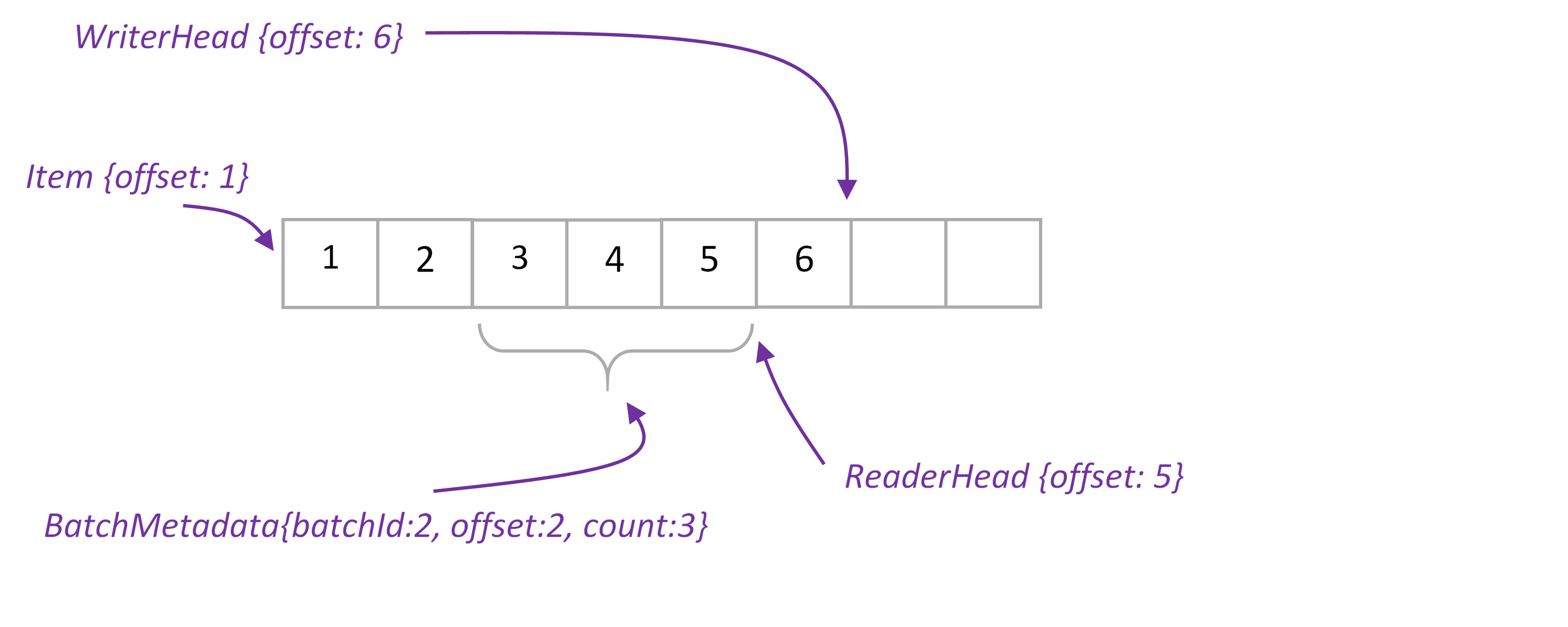
Stream’s WriterHead holds the last offset in the stream. Any time batch of elements (or single element) written to stream, WriterHead incremented by the number of elements. Allocated numbers used to populate offset property of Items. WriterHead object is kept in heap, there is no need to keep it in space. If primary partition fails, WriterHead is reinitialized to be the max offset value for given stream.
ReaderHead points to the last read item. We have to keep this value in the space, otherwise if partition fails we won’t be able to infer this value.
When spout request new batch, we take ReaderHead, read data from that point and update ReaderHead. New BatchMetadata object is placed to the space, it keeps start offset and number of items in the batch. In case Storm requests transaction replaying, we are able to reread exactly the same items by given batchId. Finally, once Storm acknowledges that batch successfully processed, we delete BatchMetadata and corresponding items from the space.
By default, Trident processes a single batch at a time, waiting for the batch to succeed or fail before trying another batch. We can get significantly higher throughput and lower latency of processing of each batch – by pipelining the batches. You configure the maximum amount of batches to be processed simultaneously with the “topology.max.spout.pending” property.
Operations with PartitionedStream are encapsulated in remote service – PartitionedStreamService.
Here is an example how to use XAPTransactionalTridentSpout:
The full example that demonstrates usage of XAPTransactionalTridentSpout to address classic Word Counter problem can be found in XAPTransactionalTridentSpoutTest.
Trident State
Trident has first-class abstractions for reading from and writing to stateful sources. Details are available on the Storm wiki site.
In Trident topology that is persisting state via this mechanism, the overall throughput is almost certainly constrained by the performance of the state persistence. This is a good place where XAP can step in and provide extremely high performance persistence for stream processing state.
XAP Trident state implementation supports all state types – non-transactional, transactional and opaque. All you need to create a Trident state is configure space url and choose appropriate factory method of XAPStateFactory class:
The full example can be found in TridentWordCountTest.
Trident Read-Only state
Trident Read-Only state allows to lookup persistent data during the computation.
Consider Twitter Reach example. Reach is the number of unique people exposed to a URL on Twitter. To compute reach, you need to fetch all the people who ever tweeted a URL, fetch all the followers of all those people, unique that set of followers, and that count that uniqued set.
XAP is a good candidate to store reference data such as tweeted url and followers. You can easily create XAP read-only state with XAPReadOnlyStateFactory. The following example demonstrates how to create a read-only state for TweeterUrl and Followers classes. The input arguments that Trident pass to stateQuery() are used as space ids.
The full example can be found in TridentReachTest.
Another option to create XAP read-only state is to use SQL query. In this case stateQuery’s input arguments are used as SQL parameters:
12
SQLQuery<Person>sqlQuery=newSQLQuery<>(Person.class,"name = ? AND age > 30").setProjections("age");TridentStatestate=topology.newStaticState(XAPReadOnlyStateFactory.bySqlQuery(sqlQuery));
The full example can be found in SqlQueryReadOnlyStateTest.
Storm bolts
If pure Storm suits better your needs, most likely you will want to read/write data from bolts to persistent storage. For instance, imagine you are processing stream of data and would like to present computation result on UI. So the final bolt in your topology pipeline should write result to XAP which can then be accessed from anywhere. For this purpose we created XAPAwareRichBolt and XAPAwareBasicBolt that have a reference to space proxy. All you need is to configure space url and extend XAP aware bolt.
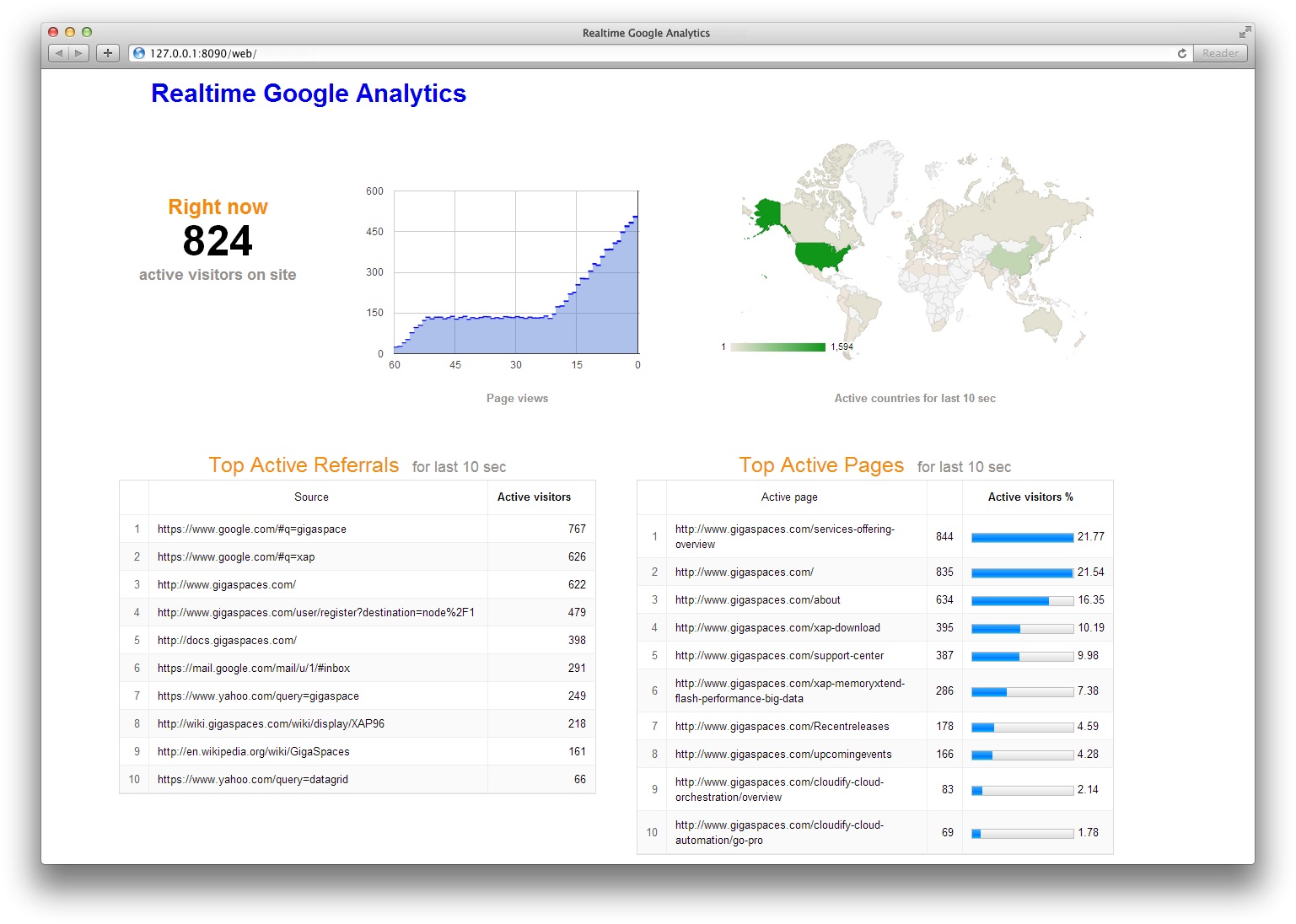
In this section we demonstrate how to build highly available, scalable equivalent of Real-time Google Analytics application and deploy it to cloud with one click using Cloudify.
Real-Time Google Analytics allows you to monitor activity as it happens on your site. The reports are updated continuously and each page view is reported seconds after it occurs on your site. For example, you can see:
how many people are on your site right now
dynamic of page views during last minute
users geographic locations
traffic sources that referred them
which pages or events they’re interacting with
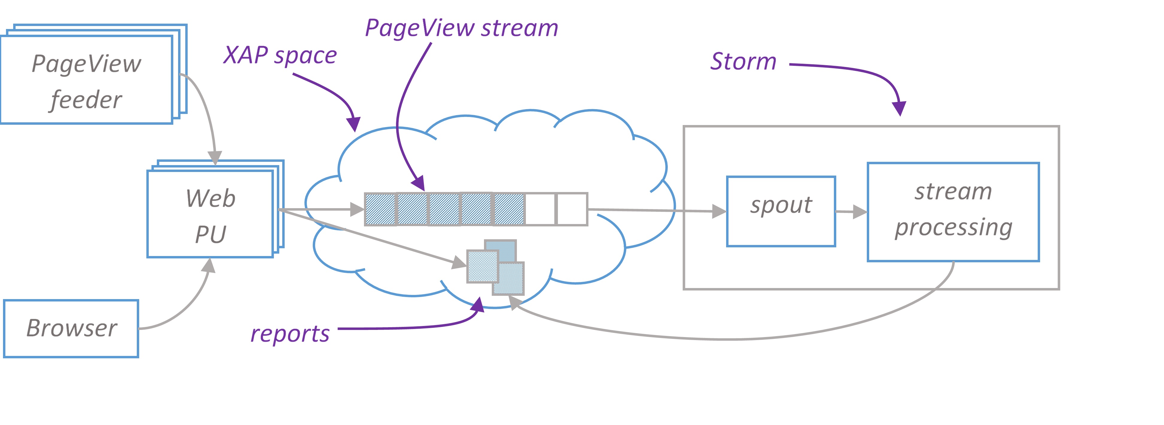
High-level architecture diagram
PageView feeder is a standalone java application that simulates users on the site. It continuously sends PageView json to rest service endpoints deployed in XAP web PU. PageView looks like this
Rest service converts JSON documents to space object and writes them to the stream. Stream is consumed by Storm topology which performs all necessary processing in memory and stores results in XAP space. End user is browsing web page hosted in Web PU that continuously updates reports with AJAX requests backed by another rest service. Rest service reads report from XAP space.
We use pure Storm to build topology. There are several reasons why we don’t use Trident for this application. We are tolerant to page views loss if some Storm node fails. We don’t need exactly-once processing semantic. Instead, we want to maximize throughput and minimize latency.
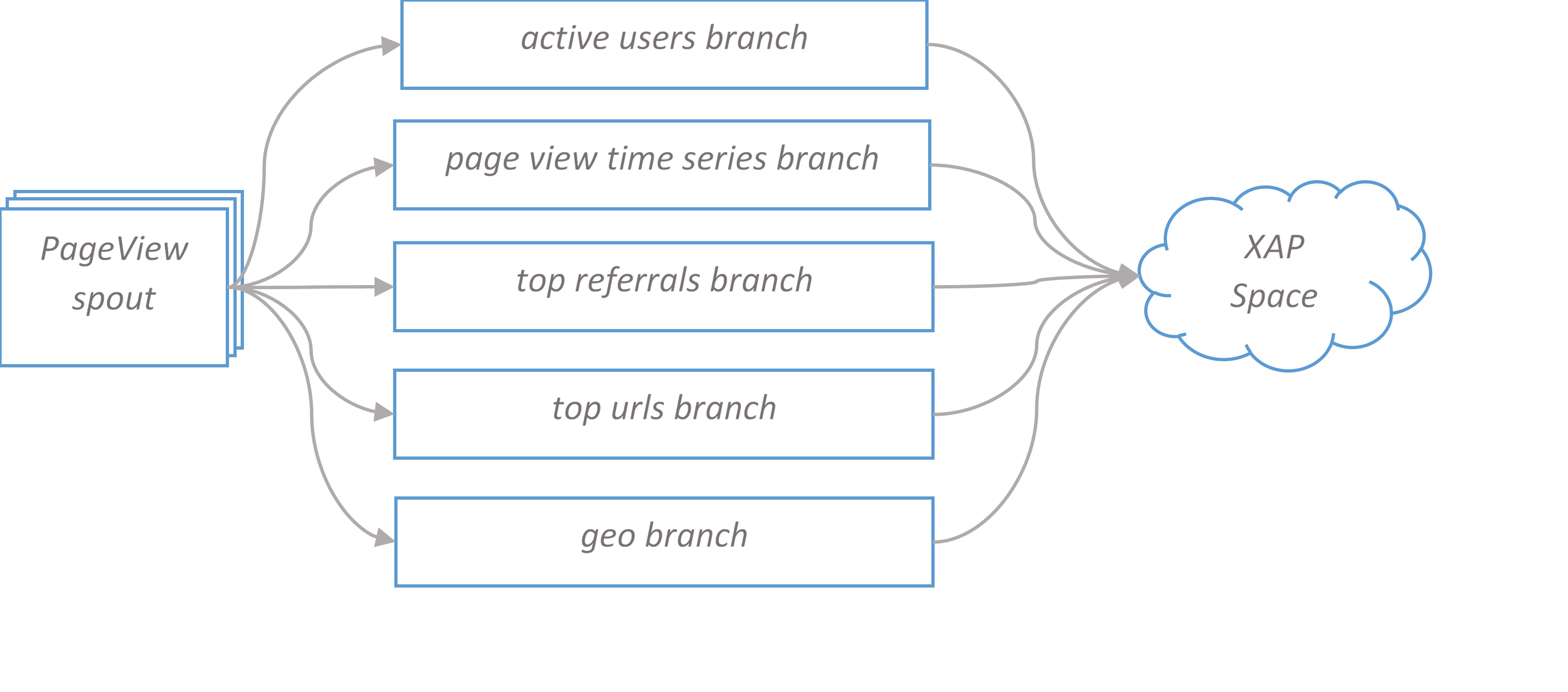
Google Analytics Topology. High level overview.
PageView spout forks five branches, each branch calculates its report and can be scaled independently. The final bolt in the branch writes data to XAP space. In the next sections we take a closer look at branches design.
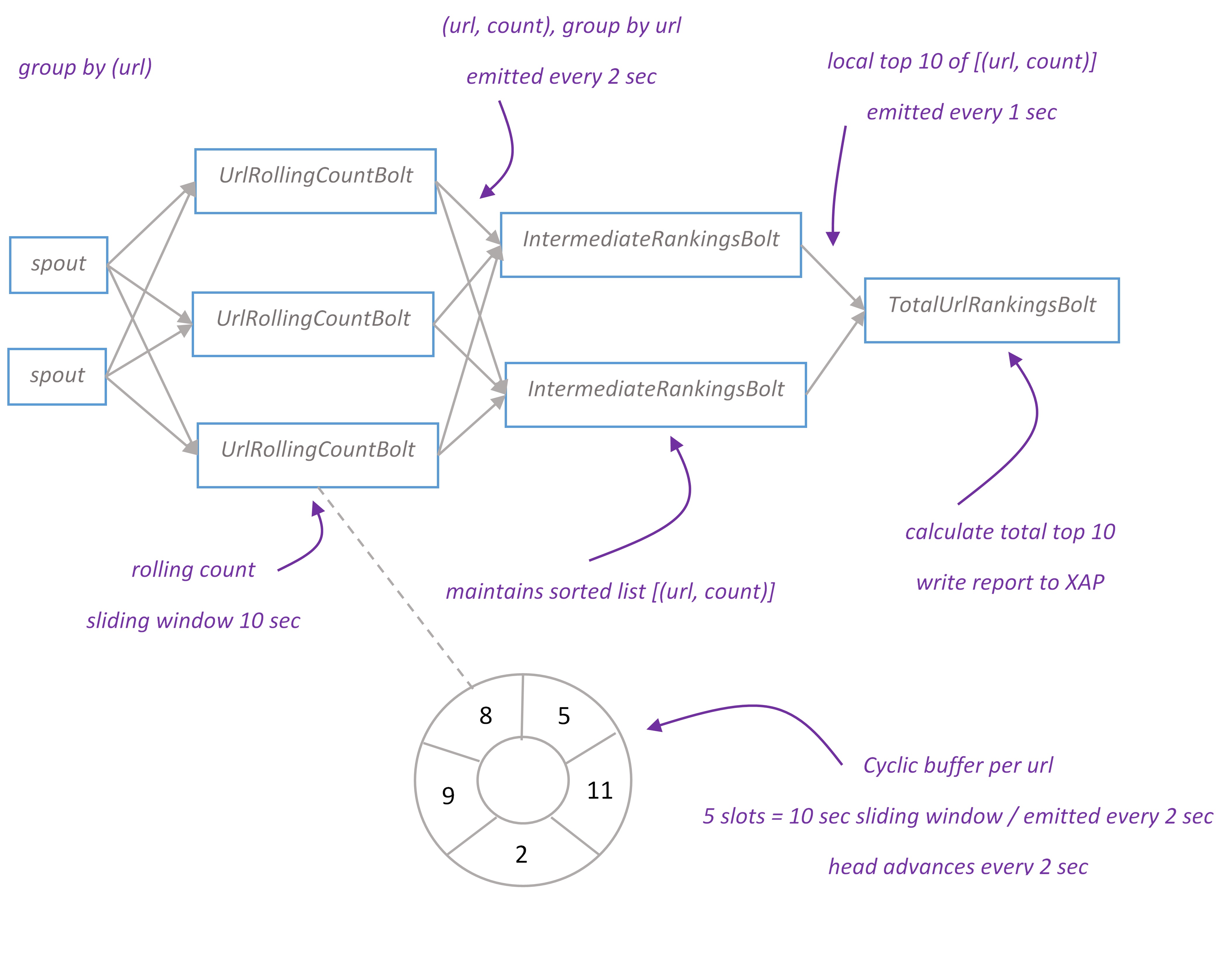
Top urls topology branch
Top urls report displays top 10 visited urls for the last ten seconds. Topology implements distributed rolling count algorithm. The report is updated every second.
Tuples flow from spout to UrlRollingCountBolt grouped by ‘url’. UrlRollingCountBolt calculates rolling count with sliding windows of 10 seconds for every url. Sliding windows is basically a cyclic buffer with a head pointing to current slot. When bolt receives new tuple, it finds a sliding window for this tuple and increments the number in current slot. Every two seconds UrlRollingCountBolt emits the sum of sliding window for every url, then sliding windows advance and head points to the next slot.
The url and its rolling count flow to IntermediateRankingsBolt which maintains pair of (url, count) in sorted by count order and emits its top 10 urls to the final stage. TotalUrlRankingBolt calculates the global top 10 urls and writes report object to XAP space. The primitives to implement rolling count algorithm can be found in storm-starter project.
Top referrals topology branch is identical to top urls one. The only difference in is that we calculate ‘referral’ rather than ‘url’ tuple field.
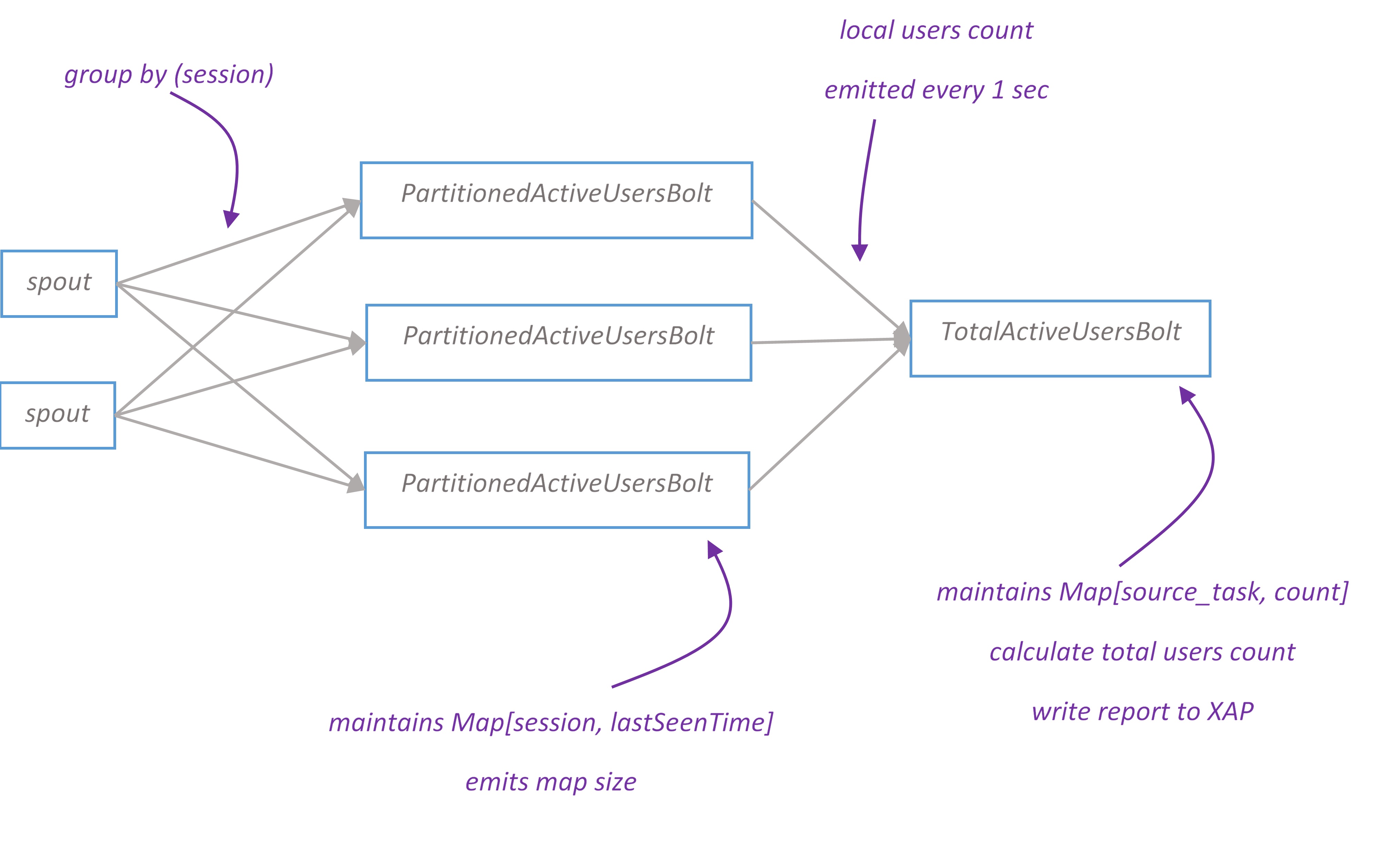
Active users topology branch
Active users report displays how many people on the site right now. We assume that if user hasn’t opened any page for the last N seconds, then user has left the site. Users are uniquely identified by ‘sessionId’ tuple field. For demo purpose N is configured to 5 seconds, though it should be much longer in real life application.
Tuples flow from spout to PartitionedActiveUsersBolt grouped by ‘sessionId’. For every sessionId PartitionedActiveUsersBolt keeps track of the last seen time. Every second it removes sessions seen last time earlier than N seconds before and then emits the number of remaining ones.
TotalActiveUsersBolt maintains a map of [source_task, count] and emits the total count for all sources. Report is written to XAP.
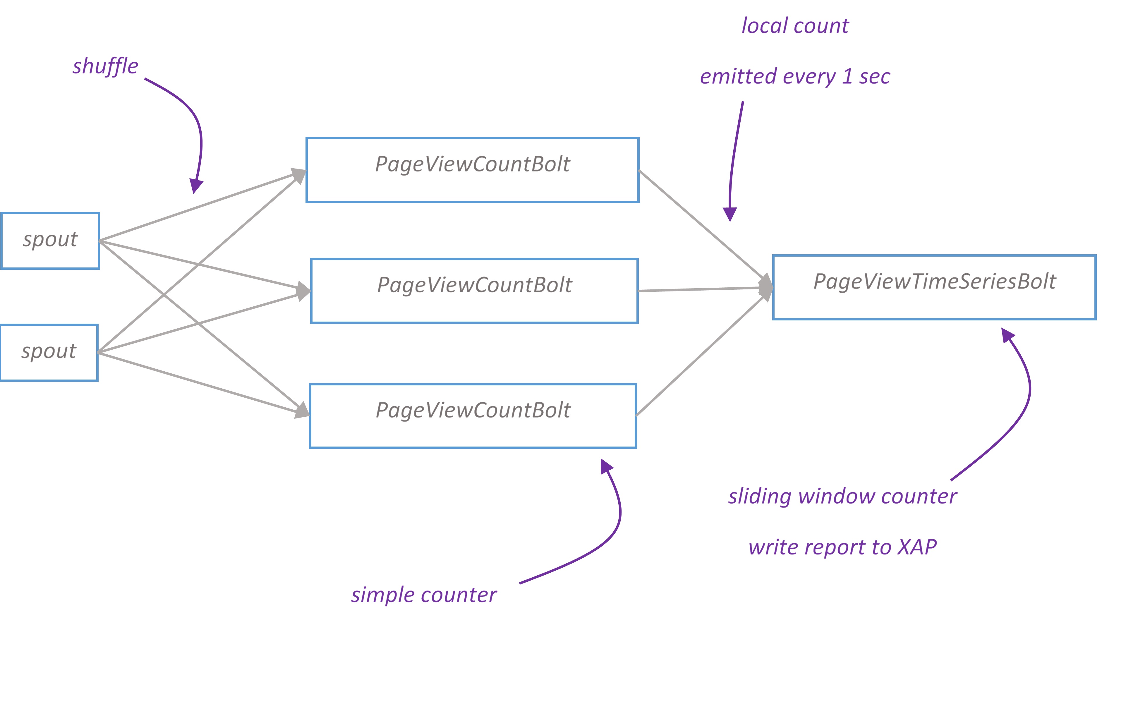
Page view time series topology branch
Page view time series report displays the dynamic of visited pages for last minute. The chart is updated every second.
PageViewCountBolt calculates the number of page views and passes local count to PageViewTimeSeriesBolt every second. PageViewTimeSeriesBolt maintains a sliding window counter and writes report to XAP space.
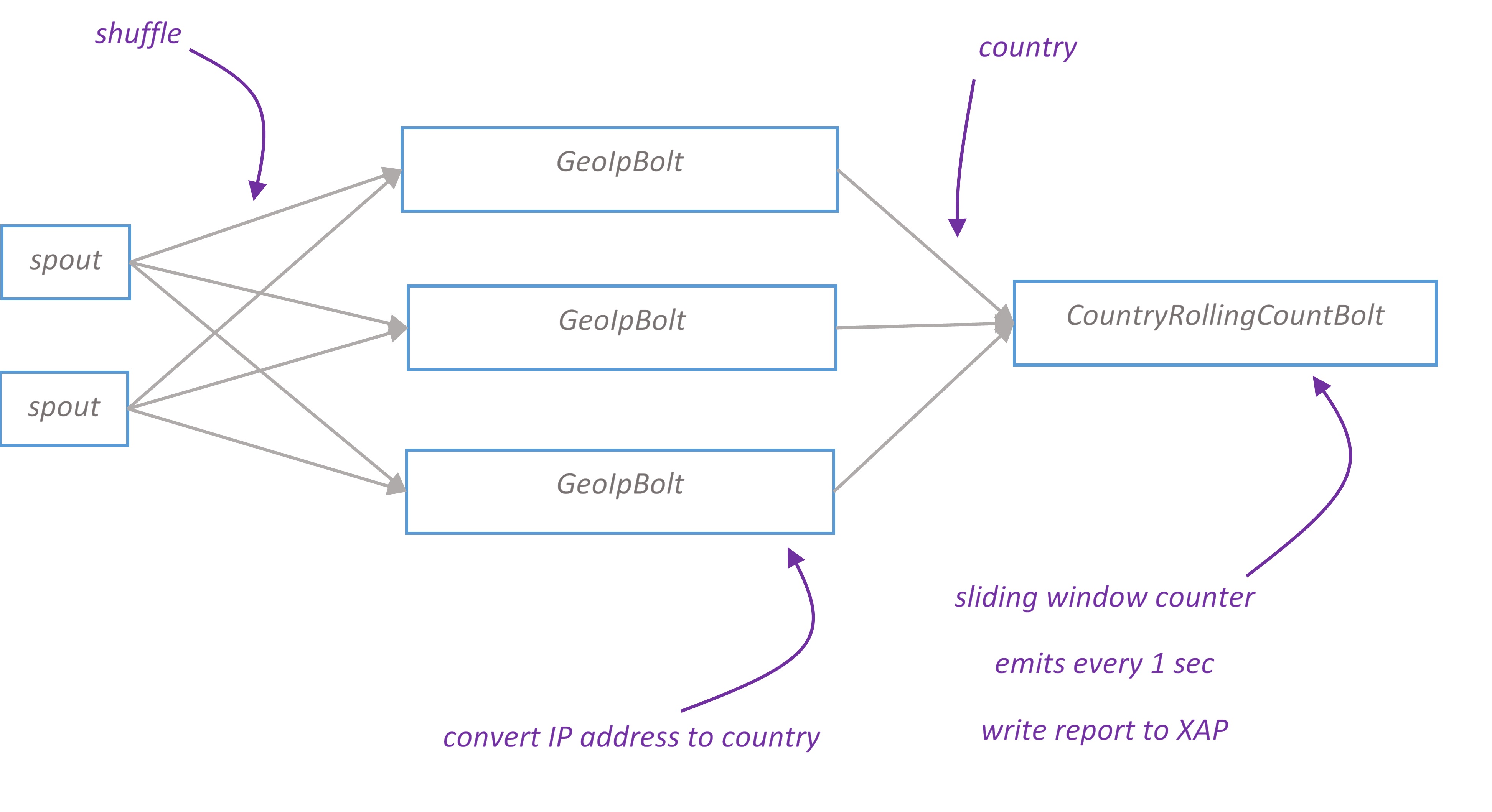
Geo topology branch
Geo report displays a map of users’ geographical location. Depending on the volume of traffic from particular country, country is filled with different colors on the map.
IP address converted to country using MaxMind GeoIP database. The database is a binary file loaded into GeoIPBolt’s heap. GeoIpLookupService ensures that it’s loaded only once per JVM.
Deploy space and Web PU by running the following from project root folder:
12
cdgoogle-analyticsmvnos:deploy
Add apache-storm-0.9.2-incubating/bin to your $PATH
Run the following to deploy topology to Storm cluster
storm jar ./storm-topology/target/storm-topology-1.0-SNAPSHOT.jar com.gigaspaces.storm.googleanalytics.topology.GoogleAnalyticsTopology google-analytics 127.0.0.1
Run feeder
java -jar ./feeder/target/feeder-1.0-SNAPSHOT.jar 127.0.0.1
Make sure that <project_root>/cloudify/apps/storm-demo/deployer/files contains up-to-date version of space-1.0.-SNAPSHOT.jar, web.war and feeder-1.0-SNAPSHOT.jar. As well as <project_root>/cloudify/apps/storm-demo/storm-nimbus/commands contains storm-topology-1.0-SNAPSHOT.jar (you can copy them from maven’s target directories using <project_root>/dev-scripts/copy-artifacts-to-cloudify.sh script)
Copy <project_root>/cloudify recipes to <cloudify_install>/recipes directory
Run cloudify <cloudify_install>/bin/cloudify.sh
Bootsrap cloud (to bootsrap local cloud, run the following in Cloudify Shell bootstrap-localcloud)
Start installation install-application storm-demo
Once installation completed, open Cloudify Management Console and check the ip address of xap-management service. Google Analytics UI should be available at http://<xap_management_service_ip>:8090/web
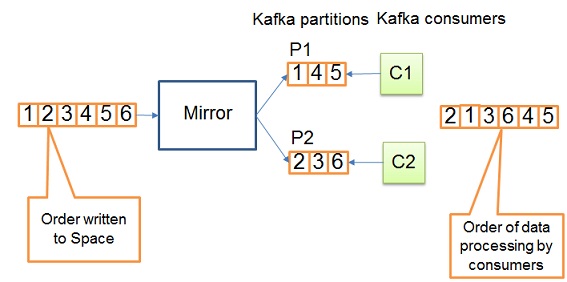
]]><![CDATA[GigaSpaces with Kafka]]>2014-05-14T16:46:56+03:00http://dyagilev.org/blog/2014/05/14/xap-kafkaApache Kafka is a distributed publish-subscribe messaging system. It is designed to support persistent messaging with a O(1) disk structures that provides constant time performance even with many TB of stored messages. Apache Kafka provides High-throughput even with very modest hardware, Kafka can support hundreds of thousands of messages per second. Apache Kafka supports partitioning the messages over Kafka servers and distributing consumption over a cluster of consumer machines while maintaining per-partition ordering semantics. Many times Apache Kafka is used to perform parallel data load into Hadoop.
This pattern integrates GigaSpaces with Apache Kafka. GigaSpaces’ write-behind IMDG operations to Kafka making it available for the subscribers. Such could be Hadoop or other data warehousing systems using the data for reporting and processing. Sources are available on github
XAP Kafka Integration Architecture
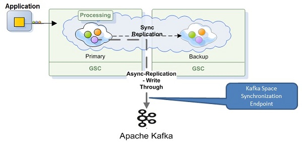
The XAP Kafka integration is done via the SpaceSynchronizationEndpoint interface deployed as a Mirror service PU. It consumes a batch of IMDG operations, converts them to custom Kafka messages and sends these to the Kafka server using the Kafka Producer API.
GigaSpace-Kafka protocol is simple and represents the data and its IMDG operation. The message consists of the IMDG operation type (Write, Update , remove, etc.) and the actual data object. The Data object itself could be represented either as a single object or as a Space Document with key/values pairs (SpaceDocument).
Since a Kafka message is sent over the wire, it should be serialized to bytes in some way.
The default encoder utilizes Java serialization mechanism which implies Space classes (domain model) to be Serializable.
By default Kafka messages are uniformly distributed across Kafka partitions. Please note, even though IMDG operations appear ordered in SpaceSynchronizationEndpoint, it doesn’t imply correct ordering of data processing in Kafka consumers. See below diagram:
Getting started
Download the Kafka Example
You can download the example code from github.
The example located under <project_root>/example. It demonstrates how to configure Kafka persistence and implements a simple Kafka consumer pulling data from Kafka and store in HsqlDB.
Running the Example
In order to run an example, please follow the instruction below:
Step 5: Check GigaSpaces log files, there should be messages from the Feeder and Consumer.
Configuration
Library Dependency
The following maven dependency needs to be included in your project in order to use Kafka persistence. This artifact is built from <project_rood>/kafka-persistence source directory.
Here is an example of the Kafka Space Synchronization Endpoint configuration:
1234567891011121314151617
<beanid="kafkaSpaceSynchronizationEndpoint"class="com.epam.openspaces.persistency.kafka.KafkaSpaceSynchronizationEndpointFactoryBean"><propertyname="producerProperties"><props><propkey="metadata.broker.list"> localhost:9092</prop><propkey="request.required.acks">1</prop></props></property></bean><!-- The mirror space. Uses the Kafka external data source. Persists changes done on the Space that connects to this mirror space into the Kafka.--><os-core:mirrorid="mirror"url="/./mirror-service"space-sync-endpoint="kafkaSpaceSynchronizationEndpoint"operation-grouping="group-by-replication-bulk"><os-core:source-spacename="space"partitions="2"backups="1"/></os-core:mirror>
Please consult Kafka documentation for the full list of available producer properties.
You can override the default properties if there is a need to customize GigaSpace-Kafka protocol. See Customization section below for details.
Space class
In order to associate a Kafka topic with the domain model class, the class needs to be annotated with the @KafkaTopic annotation and declared as Serializable. Here is an example
To configure a Kafka topic for a SpaceDocuments or Extended SpaceDocument, the property KafkaPersistenceConstants.SPACE_DOCUMENT_KAFKA_TOPIC_PROPERTY_NAME should be added to document. Here is an example
It’s also possible to configure the name of the property which defines the Kafka topic for SpaceDocuments. Set spaceDocumentKafkaTopicName to the desired value as shown below.
The Kafka persistence library provides a wrapper around the native Kafka Consumer API for the GigaSpace-Kafka protocol serialization. Please see com.epam.openspaces.persistency.kafka.consumer.KafkaConsumer, example of how to use it under <project_root>/example module.
Customization
Kafka persistence was designed to be extensible and customizable.
If you need to create a custom protocol between GigaSpace and Kafka, provide an implementation of AbstractKafkaMessage, AbstractKafkaMessageKey, AbstractKafkaMessageFactory.
If you would like to customize how data grid operations are sent to Kafka or how the Kafka topic is chosen for a given entity, provide an implementation of ‘AbstractKafkaSpaceSynchronizationEndpoint’.
If you want to create a custom serializer, look at KafkaMessageDecoder and KafkaMessageKeyDecoder.
Kafka Producer client (which is used under the hood) can be configured with a number of settings, see Kafka documentation.
]]><![CDATA[Optimization Trick]]>2014-05-13T21:48:28+03:00http://dyagilev.org/blog/2014/05/13/optimization-trickAn interesting optimization trick from Storm internals which reminded me some algorithmic problem(see in the end).
For those who haven’t heard about Storm, in short it’s a distributed realtime computation system. Scalable, fault tolerant and guarantees that every message is fully processed.
The incoming tuple(message in Storm terminology) is processed by the bolt(processing node). Bolt can spawn more tuples which in their turn are further processed by succeeding bolt(s). So you end up with a tuple tree (directed acyclic graph actually).
The question is how to guarantee that every tuple is fully processed, i.e if some bolt fails, the tuple is replayed. We have to acknowledge when intermediate tuple created and when it’s processed. With huge tuple trees, tracking the entire tree state is memory expensive.
Strom designers decided to use an elegant trick which allows to know when tuple is fully processed with O(1) memory.
Tuple is associated with a random 64bit id. The tree state is also 64bit value called ‘ack val’. Whenever tuple is created or acknowledged, just XOR tuple id with ack val. When ack val becomes 0, the tree is fully processed. Yes, there is a a small probability of mistake, at 10K acks per second, it will take 50,000,000 years until a mistake is made. And even then, it will only cause data loss if that tuple happens to fail.
Now the algorithmic problem. Given an array of integer numbers. Each number except one appears exactly twice. The remaining number appears only once in the array, find this number with one iteration and O(1) memory. Easy, yay!
]]><![CDATA[How To Decrypt Jetty's Https Tcp Dump]]>2013-03-26T16:22:03+03:00http://dyagilev.org/blog/2013/03/26/how-to-decrypt-jettys-https-tcp-dumpIf you want to capture jetty’s tcp dump of https and analyze encrypted packets later - here is an instruction. Applies for Jetty 7, not sure if the same works for other versions.
Step 1. Find obfuscated password in jetty.xml, it should start with OBF: prefix. Run it through the following deobfuscating function which I found in jetty sources.
Step 2. Now you should have the password for keystore. The location of keystore should be listed in jetty.xml. Import keys to intermediate PKCS12 format
Step 4. Now you are good to feed wireshark or other preferred tool with RSA key.
]]><![CDATA[Fractal Tree Indexes]]>2012-03-29T15:58:13+03:00http://dyagilev.org/blog/2012/03/29/fractal-tree-indexesПарни из Tokutek реализовали engine TokuDB для MySQL как замену InnoDB, улучшив производительность операций вставки, запросов и компрессии. В основе индекса лежит так называемое Fractal Tree.
Посмотрим за счет чего достигается скорость вставки и поиска по сравнению с классическим B-tree.
Асимптотическая оценка
Необходимо оговориться, что мы рассматриваем случай когда индекс хранится на диске, а не в памяти. Поэтому нас интересует оценка количества операций IO, а не операций CPU. Операции CPU занимают ничтожно малое время по сравнению с IO.
Вставка:
B-tree O((log N)/(log B))
Fractal-tree O((log N)/(B^(1-k)))
Поиск:
B-tree O((log N)/(log B))
Fractal-tree O((log N)/(log (k*B^(1-k)))
где B - размер IO блока
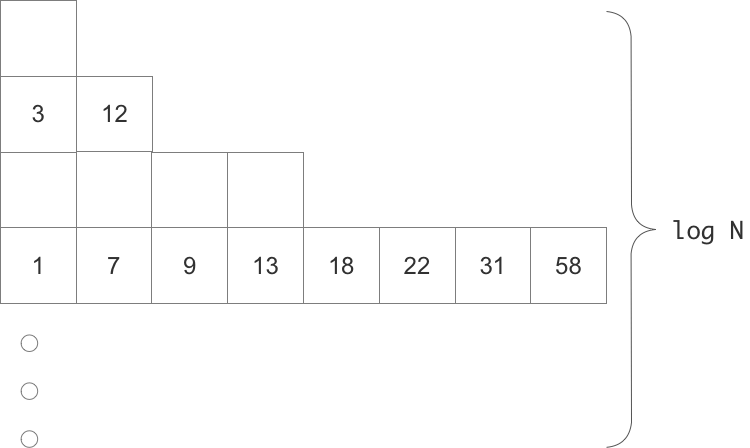
Итак, упрощенный вариант Fractal Tree:
log N массивов размером 2^i
каждый массив или полностью пустой или полностью заполнен
каждый массив отсортирован
Вставка
Начинаем сверху. Смотрим на верхний массив размером 1. Если он пустой - кладем туда элемент. Иначе вынимаем элемент и сортируем с данным во временом массиве. Спускаемся вниз к массиву размером 2. Если он пустой - кладем туда нашу пару. Если нет - мержим их с временным массивом. Так как оба массива отсортированы, то делаем ето за O(X), где X ето длина массива. По сути ето операция merge из merge-сортировки.
Амортизированное время вставки занимает O((log N)/B), хотя в худшем случае вставка одного элемента может повлечь за собой перезапись огромного количества данных по цепочке. Чтобы избежать пиков с длительным ответом TokuDB порождает отдельный поток для вставки, ответ для клиента возвращается немедленно.
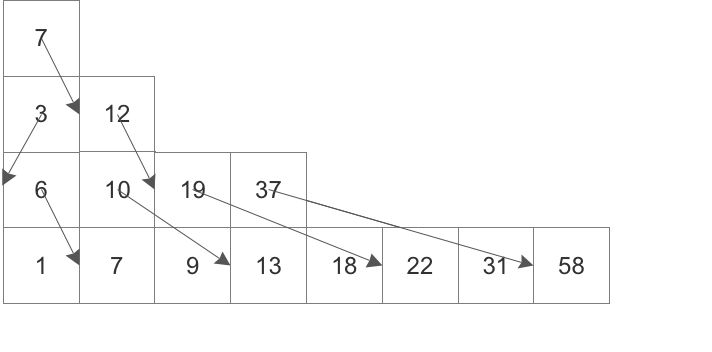
Поиск
проходимся по массивам, в кажом массиве используем бинарный поиск. Итого - O((log N)^2). Это медленнее чем B-tree. Как это можно ускорить?
Идея состоит в том, чтобы во время поиска в очередном массиве использовать некоторую информацию из поиска предыдущего массива. И так по цепочке. А информация следующая - каждый элемент массива хранит ссылку на его ‘виртуальное’ место в следующем массиве. Называется ето fractional cascading.
Итого, log N массивов, константное время на каждом массиве дает O(log N).
В целом товарищи из Tokutek считают что в будущем все перейдут на фрактальные деревья как замена Б-деревьям. Детали алгоритма запатентованы.
]]><![CDATA[Consistent Hashing]]>2012-03-23T15:34:54+03:00http://dyagilev.org/blog/2012/03/23/consistent-hashingТехника консистентного хеширования consistent hashing довольно популярна при создании распределенных систем, тем не менее я не смог найти описания алгоритма на русском языке. Попробую изложить, возможно кому-то пригодится.
Проблема
Предположим вы разрабатываете приложение и решили кешировать данные для улучшения производительности. Так же вы решили использовать горизонтальное масштабирование и разнести данные на N серверов.
Итого, есть N серверов и необходимо реализовать две функции:
12
voidput(Keyk,Itemi)// положить элемент i с ключом k в кешItemget(Keyk);// вытащить элемент по ключу k
Имея ключ k, как узнать на каком сервере лежит соответствующий ему элемент?
Решение
Первое что приходит в голову - использовать обычную хеш-таблицу. Берем ключ k, применяем к нему хеш-функцию и считаем остаток от деления на количество серверов N - hash(k) mod N. Да, это будет работать, но что произойдет когда мы захотим добавить ещё один сервер ? Нам необходимо будет перехешировать все данные, большую часть которых нужно будет загрузить на новые сервера. Это дорогая операция. Также не понятно что делать в случае падения существующего сервера.
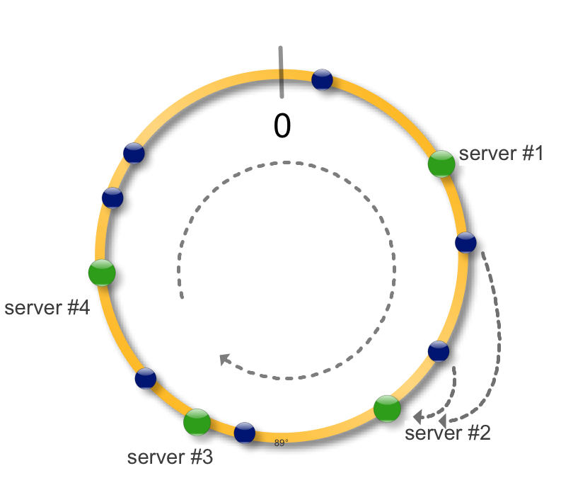
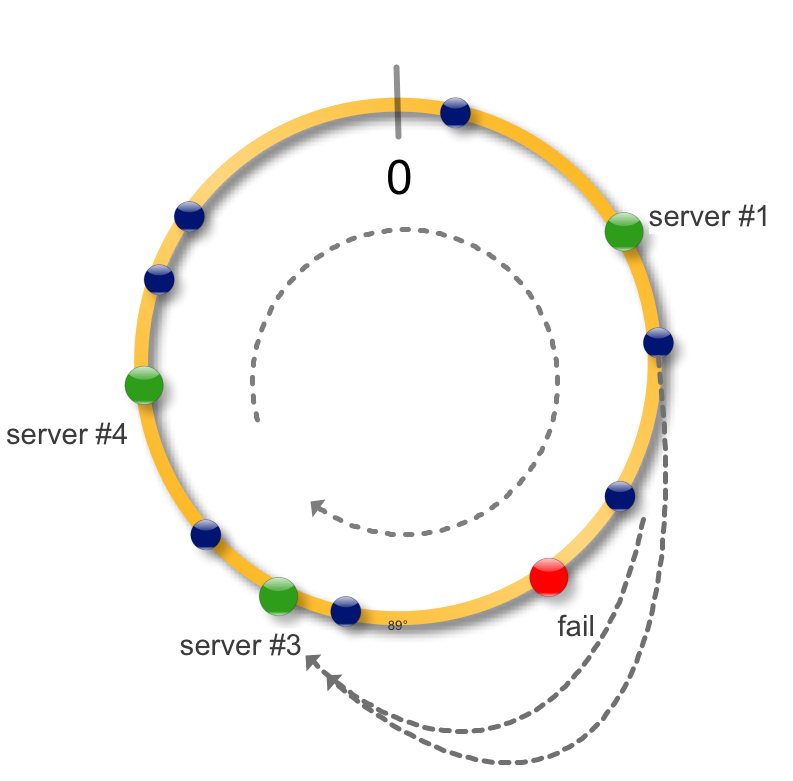
Здесь появляется консистентное кеширование. Идея простая, возьмем окружность и будем рассматривать ее как интервал на котором определена хеш-функция функция. Применив хеш-функцию к набору ключей (синие точки) и серверов (зеленые точки) сможем разместить их на окружности.
Для того чтобы определить на каком сервере размещен ключ, найдем ключ на окружности и будем двигаться по часовой стрелке до ближайшего сервера.
Теперь в случае падения (недоступности) сервера, загрузить на новые сервер необходимо только недоступные данные. Все остальные хеши не меняют свое местоположение, то есть консистенты.
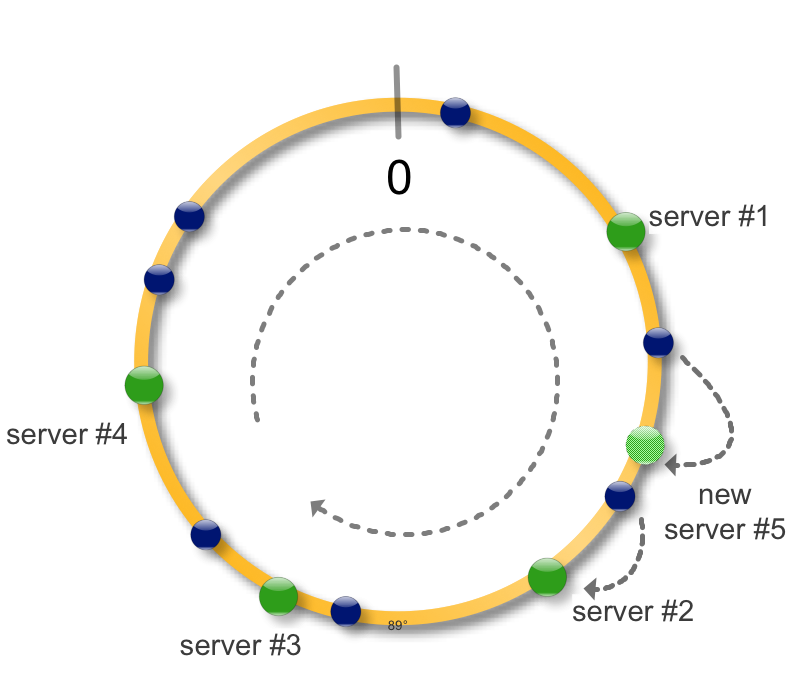
При добавлении нового сервера соседний разделяет с ним часть своих данных.
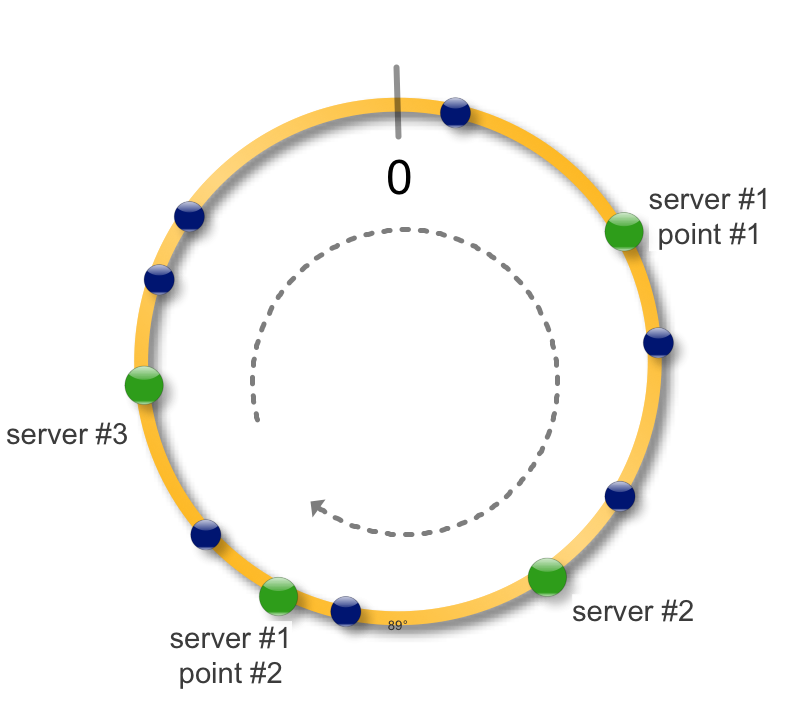
В целом ето все. На практике также применяют следующий трюк. Сервер можно пометить на окружности не одной точкой, а несколькими.
Что ето дает ?
- более равномерное распределение данных по серверам
- при падении сервера данные распределяются не на один соседний, а на несколько, распределяя тем самым нагрузку
- при добавлении нового сервера, точки можно делать ‘активными’ постепенно одна за другой, предотвращая шквальную нагрузку на сервер
- если конфигурация серверов отличается, например размером диска, количество данных можно контролировать числом его точек. Больше точек - большая длина окружности принадлежит етому серверу и соответственно больше данных.
Реализация
Храним хеши серверов в виде какого-либо дерева, например Red-Black. Операция поиска сервера по ключу будет занимать O(log n).
]]><![CDATA[Code Refactoring Detection]]>2012-03-21T15:13:35+03:00http://dyagilev.org/blog/2012/03/21/code-refactoring-detectionAn idea of feature I would love to see in code review and diff/merge tools.
Consider you are reviewing code changes or making 3-way merge where among various things a name of some method has changed. Personally I don’t want to go through tens of files and check that all usages of method changed accordingly.
I would like to see it in more declarative way. One phrase saying ‘method Foo.bar() has changed to Foo.bar2()’ would be enough. Imagine you could accept this particular change and now tool ignores it making the whole picture clearer.
Say for static object-oriented languages I can imagine a number of refactoring types where this could be useful - method extract, all kind of renames, replacing inheritance with delegation, replacing constructor with factory methods and so on.
How difficult would it be to implement semantic aware diff on top of Intellij IDEA ?
]]><![CDATA[Hello Blog]]>2012-03-21T14:11:52+03:00http://dyagilev.org/blog/2012/03/21/helloThis blog is my shady nook to write some random thoughts on computer science and related topics.
]]>