Shady Minds

Oleksii Diagiliev on computer science and related ..

Scalable machine learning with InsightEdge: mobile advertisement clicks prediction

This blog post will provide an introduction into using machine learning algorithms with InsightEdge. We will go through an exercise to predict mobile advertisement click-through rate with Avazu’s dataset.

Overview

There are several compensation models in online advertising industry, probably the most notable is CPC (Cost Per Click), in which an advertiser pays a publisher when the ad is clicked. Search engine advertising is one of the most popular forms of CPC. It allows advertisers to bid for ad placement in a search engine’s sponsored links when someone searches on a keyword that is related to their business offering.

For the search engines like Google, advertising is one of the main sources of their revenue. The challenge for the advertising system is to determine what ad should be displayed for each query that the search engine receives.

The revenue search engine can get is essentially:

revenue = bid * probability_of_click

The goal is to maximize the revenue for every search engine query. Whereis the bid is a known value, the probability_of_click is not. Thus predicting the probability of click becomes the key task.

Working on a machine learning problem involves a lot of experiments with feature selection, feature transformation, training different models and tuning parameters.While there are a few excellent machine learning libraries for Python and R, like scikit-learn, their capabilities are typically limited to relatively small datasets that you fit on a single machine.

With the large datasets and/or CPU intensive workloads you may want to scale out beyond a single machine. This is one of the key benefits of InsightEdge, since it’s able to scale the computation and data storage layers across many machines under one unified cluster.

Loading the data

The dataset consists of:

  • train (5.9G) - Training set. 10 days of click-through data, ordered chronologically. Non-clicks and clicks are subsampled according to different strategies.
  • test (674M) - Test set. 1 day of ads to test model predictions.

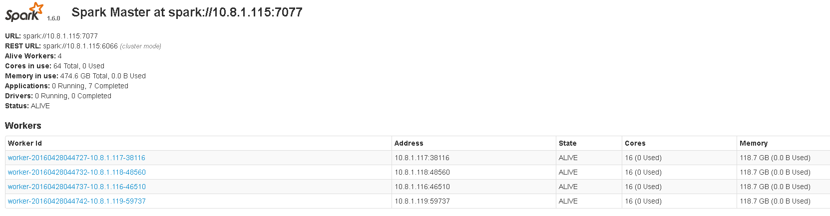
At first, we want to launch InsightEdge.

To get the first data insights quickly, one can launch InsightEdge on a laptop. Though for the big datasets or compute-intensive tasks the resources of a single machine might not be enough.

For this problem we will setup a cluster with four workers and place the downloaded files on HDFS.

Let’s open the interactive Web Notebook and start exploring our dataset.

The dataset is in csv format, so we will use databricks csv library to load it from hdfs into the Spark dataframe:

1
2
%dep
z.load("com.databricks:spark-csv_2.10:1.3.0")

Load the dataframe into Spark memory and cache:

1
2
3
4
5
6
7
val df = sqlContext.read
      .format("com.databricks.spark.csv")
      .option("header", "true")
      .option("inferSchema", "false")
      .load("hdfs://10.8.1.116/data/avazu_ctr/train")

df.cache()

Exploring the data

Now that we have the dataset in Spark memory, we can read the first rows:

1
df.show(10)
1
2
3
4
5
6
7
8
9
10
11
12
13
14
15
+--------------------+-----+--------+----+----------+--------+-----------+-------------+--------+----------+------------+---------+---------+------------+-----------+----------------+-----+---+---+----+---+---+------+---+
|                  id|click|    hour|  C1|banner_pos| site_id|site_domain|site_category|  app_id|app_domain|app_category|device_id|device_ip|device_model|device_type|device_conn_type|  C14|C15|C16| C17|C18|C19|   C20|C21|
+--------------------+-----+--------+----+----------+--------+-----------+-------------+--------+----------+------------+---------+---------+------------+-----------+----------------+-----+---+---+----+---+---+------+---+
| 1000009418151094273|    0|14102100|1005|         0|1fbe01fe|   f3845767|     28905ebd|ecad2386|  7801e8d9|    07d7df22| a99f214a| ddd2926e|    44956a24|          1|               2|15706|320| 50|1722|  0| 35|    -1| 79|
|10000169349117863715|    0|14102100|1005|         0|1fbe01fe|   f3845767|     28905ebd|ecad2386|  7801e8d9|    07d7df22| a99f214a| 96809ac8|    711ee120|          1|               0|15704|320| 50|1722|  0| 35|100084| 79|
|10000371904215119486|    0|14102100|1005|         0|1fbe01fe|   f3845767|     28905ebd|ecad2386|  7801e8d9|    07d7df22| a99f214a| b3cf8def|    8a4875bd|          1|               0|15704|320| 50|1722|  0| 35|100084| 79|
|10000640724480838376|    0|14102100|1005|         0|1fbe01fe|   f3845767|     28905ebd|ecad2386|  7801e8d9|    07d7df22| a99f214a| e8275b8f|    6332421a|          1|               0|15706|320| 50|1722|  0| 35|100084| 79|
|10000679056417042096|    0|14102100|1005|         1|fe8cc448|   9166c161|     0569f928|ecad2386|  7801e8d9|    07d7df22| a99f214a| 9644d0bf|    779d90c2|          1|               0|18993|320| 50|2161|  0| 35|    -1|157|
|10000720757801103869|    0|14102100|1005|         0|d6137915|   bb1ef334|     f028772b|ecad2386|  7801e8d9|    07d7df22| a99f214a| 05241af0|    8a4875bd|          1|               0|16920|320| 50|1899|  0|431|100077|117|
|10000724729988544911|    0|14102100|1005|         0|8fda644b|   25d4cfcd|     f028772b|ecad2386|  7801e8d9|    07d7df22| a99f214a| b264c159|    be6db1d7|          1|               0|20362|320| 50|2333|  0| 39|    -1|157|
|10000918755742328737|    0|14102100|1005|         1|e151e245|   7e091613|     f028772b|ecad2386|  7801e8d9|    07d7df22| a99f214a| e6f67278|    be74e6fe|          1|               0|20632|320| 50|2374|  3| 39|    -1| 23|
|10000949271186029916|    1|14102100|1005|         0|1fbe01fe|   f3845767|     28905ebd|ecad2386|  7801e8d9|    07d7df22| a99f214a| 37e8da74|    5db079b5|          1|               2|15707|320| 50|1722|  0| 35|    -1| 79|
|10001264480619467364|    0|14102100|1002|         0|84c7ba46|   c4e18dd6|     50e219e0|ecad2386|  7801e8d9|    07d7df22| c357dbff| f1ac7184|    373ecbe6|          0|               0|21689|320| 50|2496|  3|167|100191| 23|
+--------------------+-----+--------+----+----------+--------+-----------+-------------+--------+----------+------------+---------+---------+------------+-----------+----------------+-----+---+---+----+---+---+------+---+
only showing top 10 rows

The data fields are:

  • id: ad identifier
  • click: 0/1 for non-click/click
  • hour: format is YYMMDDHH
  • C1: anonymized categorical variable
  • banner_pos
  • site_id
  • site_domain
  • site_category
  • app_id
  • app_domain
  • app_category
  • device_id
  • device_ip
  • device_model
  • device_type
  • device_conn_type
  • C14-C21 – anonymized categorical variables

Let’s see how many rows are in the training dataset:

1
2
3
val totalCount = df.count()

totalCount: Long = 40428967

There are about 40M+ rows in the dataset.

Let’s now calculate the CTR (click-through rate) of the dataset. The click-through rate is the number of times a click is made on the advertisement divided by the total impressions (the number of times an advertisement was served):

1
2
3
4
5
val clicks = df.filter("click = 1").count()
val ctr = clicks.toFloat / totalCount

clicks: Long = 6865066
ctr: Float = 0.16980562

The CTR is 0.169 (or 16.9%) which is quite a high number, the common value in the industry is about 0.2-0.3%. So a high value is probably because non-clicks and clicks are subsampled according to different strategies, as stated by Avazu.

Now, the question is which features should we use to create a predictive model? This is a difficult question that requires a deep knowledge of the problem domain. Let’s try to learn it from the dataset we have.

For example, let’s explore the device_conn_type feature. Our assumption might be that this is a categorical variable like Wi-Fi, 2G, 3G or LTE. This might be a relevant feature since clicking on an ad with a slow connection is not something common.

At first, we register the dataframe as a SQL table:

1
df.registerTempTable("training")

and run the SQL query:

1
2
3
4
%sql
SELECT device_conn_type, SUM(click) as clicks_num, COUNT(click) as impression, SUM(click)/COUNT(click) as ctr
FROM training
GROUP BY device_conn_type

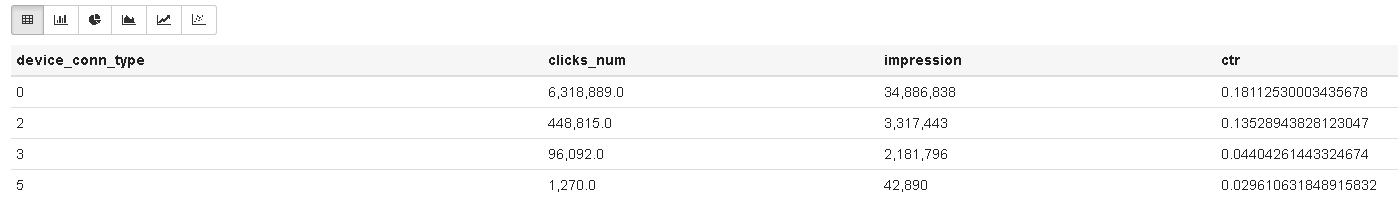
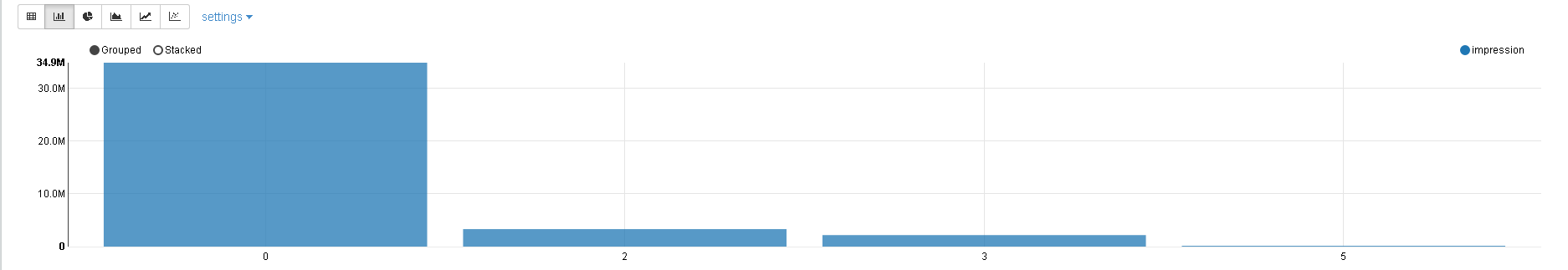
We see that there are four connection type categories. Two categories with CTR 18% and 13%, and the first one is almost 90% of the whole dataset. The other two categories have significantly lower CTR.

Another observation we may notice is that features C15 and C16 look like the ad size:

1
2
3
4
5
%sql
SELECT C15, C16, COUNT(click) as impression, SUM(click)/COUNT(click) as ctr
FROM training
GROUP BY C15, C16
ORDER BY ctr DESC

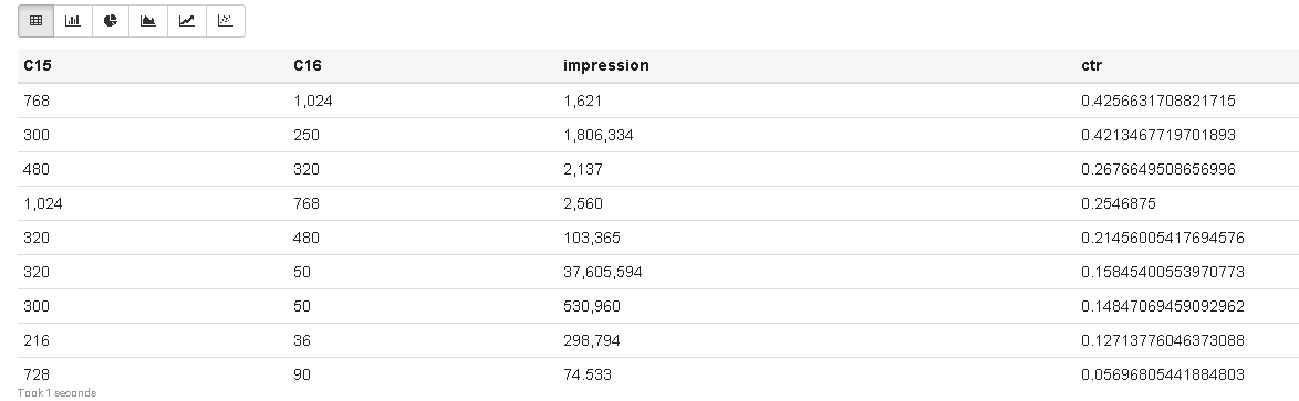
We can notice some correlation between the ad size and its performance. The most common one appears to be 320x50px known as “mobile leaderboard” in Google AdSense.

What about other features? All of them represent categorical values, how many unique categories for each feature?

1
2
3
df.columns.map(c => (c, df.select(c).distinct().count()))

res14: Array[(String, Long)] = Array((id,40428967), (click,2), (hour,240), (C1,7), (banner_pos,7), (site_id,4737), (site_domain,7745), (site_category,26), (app_id,8552), (app_domain,559), (app_category,36), (device_id,2686408), (device_ip,6729486), (device_model,8251), (device_type,5), (device_conn_type,4), (C14,2626), (C15,8), (C16,9), (C17,435), (C18,4), (C19,68), (C20,172), (C21,60))

We see that there are some features with a lot of unique values, for example, device_ip has 6M+ different values. Machine learning algorithms are typically defined in terms of numerical vectors rather than categorical values. Converting such categorical features will result in a high dimensional vector which might be very expensive. We will need to deal with this later.

Processing and transforming the data

Looking further at the dataset, we can see that the hour feature is in YYMMDDHH format. To allow the predictive model to effectively learn from this feature it makes sense to transform it into three features: year, month and hour. Let’s develop the function to transform the dataframe:

1
2
3
4
5
6
7
8
9
10
11
12
13
14
15
16
17
18
19
20
21
22
23
24
25
26
27
28
29
import java.text.SimpleDateFormat
import java.util.{Calendar, Date}
import org.apache.spark.sql.DataFrame

object DateUtils {
  val dateFormat = new ThreadLocal[SimpleDateFormat]() {
    override def initialValue(): SimpleDateFormat = new SimpleDateFormat("yyMMddHH")
  }

  def parse(s: String, field: Int): Int = {
    val date = dateFormat.get().parse(s)
    val cal = Calendar.getInstance()
    cal.setTime(date)
    cal.get(field)
  }
}

def transformHour(df: DataFrame): DataFrame = {
  val toYear = udf[Int, String](s => DateUtils.parse(s, Calendar.YEAR))
  val toMonth = udf[Int, String](s => DateUtils.parse(s, Calendar.MONTH))
  val toDay = udf[Int, String](s => DateUtils.parse(s, Calendar.DAY_OF_MONTH))
  val toHour = udf[Int, String](s => DateUtils.parse(s, Calendar.HOUR_OF_DAY))

  df.withColumn("time_year", toYear(df("hour")))
  .withColumn("time_month", toMonth(df("hour")))
  .withColumn("time_day", toDay(df("hour")))
  .withColumn("time_hour", toHour(df("hour")))
  .drop("hour")
}

We can now apply this transformation to our dataframe and see the result:

1
2
3
val hourDecoded = transformHour(df)
hourDecoded.cache()
hourDecoded.show(10)
1
2
3
4
5
6
7
8
9
10
11
12
13
14
+--------------------+-----+----+----------+--------+-----------+-------------+--------+----------+------------+---------+---------+------------+-----------+----------------+-----+---+---+----+---+---+------+---+---------+----------+--------+---------+
|                  id|click|  C1|banner_pos| site_id|site_domain|site_category|  app_id|app_domain|app_category|device_id|device_ip|device_model|device_type|device_conn_type|  C14|C15|C16| C17|C18|C19|   C20|C21|time_year|time_month|time_day|time_hour|
+--------------------+-----+----+----------+--------+-----------+-------------+--------+----------+------------+---------+---------+------------+-----------+----------------+-----+---+---+----+---+---+------+---+---------+----------+--------+---------+
| 1000009418151094273|    0|1005|         0|1fbe01fe|   f3845767|     28905ebd|ecad2386|  7801e8d9|    07d7df22| a99f214a| ddd2926e|    44956a24|          1|               2|15706|320| 50|1722|  0| 35|    -1| 79|     2014|         9|      21|        0|
|10000169349117863715|    0|1005|         0|1fbe01fe|   f3845767|     28905ebd|ecad2386|  7801e8d9|    07d7df22| a99f214a| 96809ac8|    711ee120|          1|               0|15704|320| 50|1722|  0| 35|100084| 79|     2014|         9|      21|        0|
|10000371904215119486|    0|1005|         0|1fbe01fe|   f3845767|     28905ebd|ecad2386|  7801e8d9|    07d7df22| a99f214a| b3cf8def|    8a4875bd|          1|               0|15704|320| 50|1722|  0| 35|100084| 79|     2014|         9|      21|        0|
|10000640724480838376|    0|1005|         0|1fbe01fe|   f3845767|     28905ebd|ecad2386|  7801e8d9|    07d7df22| a99f214a| e8275b8f|    6332421a|          1|               0|15706|320| 50|1722|  0| 35|100084| 79|     2014|         9|      21|        0|
|10000679056417042096|    0|1005|         1|fe8cc448|   9166c161|     0569f928|ecad2386|  7801e8d9|    07d7df22| a99f214a| 9644d0bf|    779d90c2|          1|               0|18993|320| 50|2161|  0| 35|    -1|157|     2014|         9|      21|        0|
|10000720757801103869|    0|1005|         0|d6137915|   bb1ef334|     f028772b|ecad2386|  7801e8d9|    07d7df22| a99f214a| 05241af0|    8a4875bd|          1|               0|16920|320| 50|1899|  0|431|100077|117|     2014|         9|      21|        0|
|10000724729988544911|    0|1005|         0|8fda644b|   25d4cfcd|     f028772b|ecad2386|  7801e8d9|    07d7df22| a99f214a| b264c159|    be6db1d7|          1|               0|20362|320| 50|2333|  0| 39|    -1|157|     2014|         9|      21|        0|
|10000918755742328737|    0|1005|         1|e151e245|   7e091613|     f028772b|ecad2386|  7801e8d9|    07d7df22| a99f214a| e6f67278|    be74e6fe|          1|               0|20632|320| 50|2374|  3| 39|    -1| 23|     2014|         9|      21|        0|
|10000949271186029916|    1|1005|         0|1fbe01fe|   f3845767|     28905ebd|ecad2386|  7801e8d9|    07d7df22| a99f214a| 37e8da74|    5db079b5|          1|               2|15707|320| 50|1722|  0| 35|    -1| 79|     2014|         9|      21|        0|
|10001264480619467364|    0|1002|         0|84c7ba46|   c4e18dd6|     50e219e0|ecad2386|  7801e8d9|    07d7df22| c357dbff| f1ac7184|    373ecbe6|          0|               0|21689|320| 50|2496|  3|167|100191| 23|     2014|         9|      21|        0|
+--------------------+-----+----+----------+--------+-----------+-------------+--------+----------+------------+---------+---------+------------+-----------+----------------+-----+---+---+----+---+---+------+---+---------+----------+--------+---------+

It looks like the year and month have only one value, let’s verify it:

1
2
3
4
5
hourDecoded.select("time_month").distinct.count()
hourDecoded.select("time_year").distinct.count()

res20: Long = 1
res21: Long = 1

We can safely drop these columns as they don’t bring any knowledge to our model:

1
val hourDecoded2 = hourDecoded.drop("time_month").drop("time_year")

Let’s also convert click from String to Double type.

1
2
3
4
5
6
import org.apache.spark.sql.types.DoubleType

val prepared = hourDecoded2
    .withColumn("clickTmp", hourDecoded2("click").cast(DoubleType))
    .drop("click")
    .withColumnRenamed("clickTmp", "click")

Saving preprocessed data to the data grid

The entire training dataset contains 40M+ rows, it takes quite a long time to experiment with different algorithms and approaches even in a clustered environment. We want to sample the dataset and checkpoint it to the in-memory data grid that is running collocated with Spark. This way we can: * quickly iterate through different approaches * restart the Zeppelin session or launch other Spark applications and pick up the dataset more quickly from memory

Since the training dataset contains the data for the 10 days, we can pick any day and sample it:

1
2
3
prepared.filter("time_day = 21").count()

res51: Long = 4122995

There are 4M+ rows for this day, which is about 10% of the entire dataset.

Now let’s save it to the data grid. This can be done with two lines of code:

1
2
import org.apache.spark.sql.insightedge._
prepared.filter("time_day = 21").write.grid.save("day_21")

Any time later in another Spark context we can bring the collection to the Spark memory with:

1
val df = sqlContext.read.grid.load("day_21")

Also, we want to transform the test dataset that we will use for prediction in a similar way.

1
2
3
4
5
6
7
8
9
10
val testDf = sqlContext.read
      .format("com.databricks.spark.csv")
      .option("header", "true")
      .option("inferSchema", "false")
      .load("hdfs://10.8.1.116/data/avazu_ctr/test")

transformHour(testDf)
    .drop("time_month")
    .drop("time_year")
    .write.grid.save("test")

The complete listing of notebook can be found on github. You can import it to Zeppelin and play with it on your own.

A simple algorithm

Now that we have training and test datasets sampled, initially preprocessed and available in the data grid, we can close Web Notebook and start experimenting with different techniques and algorithms by submitting Spark applications.

For our first baseline approach let’s take a single feature device_conn_type and logistic regression algorithm:

1
2
3
4
5
6
7
8
9
10
11
12
13
14
15
16
17
18
19
20
21
22
23
24
25
26
27
28
29
30
31
32
33
34
35
36
37
38
39
40
41
42
43
44
45
46
47
48
49
50
51
52
53
54
55
56
57
58
59
60
61
62
63
64
65
66
67
68
69
70
71
72
73
74
75
import com.gigaspaces.spark.context.GigaSpacesConfig
import com.gigaspaces.spark.implicits._
import org.apache.spark.ml.feature.{OneHotEncoder, StringIndexer}
import org.apache.spark.mllib.classification.LogisticRegressionWithLBFGS
import org.apache.spark.mllib.evaluation.BinaryClassificationMetrics
import org.apache.spark.mllib.linalg.Vector
import org.apache.spark.mllib.regression.LabeledPoint
import org.apache.spark.sql.SQLContext
import org.apache.spark.sql.insightedge._
import org.apache.spark.{SparkConf, SparkContext}

object CtrDemo1 {

  def main(args: Array[String]): Unit = {
    if (args.length < 3) {
      System.err.println("Usage: CtrDemo1 <spark master url> <grid locator> <train collection>")
      System.exit(1)
    }

    val Array(master, gridLocator, trainCollection) = args

    // Configure InsightEdge settings
    val gsConfig = GigaSpacesConfig("insightedge-space", None, Some(gridLocator))
    val sc = new SparkContext(new SparkConf().setAppName("CtrDemo1").setMaster(master).setGigaSpaceConfig(gsConfig))
    val sqlContext = new SQLContext(sc)

    // load training collection from data grid
    val trainDf = sqlContext.read.grid.load(trainCollection)
    trainDf.cache()

    // use one-hot-encoder to convert 'device_conn_type' categorical feature into a vector
    val indexed = new StringIndexer()
      .setInputCol("device_conn_type")
      .setOutputCol("device_conn_type_index")
      .fit(trainDf)
      .transform(trainDf)

    val encodedDf = new OneHotEncoder()
      .setDropLast(false)
      .setInputCol("device_conn_type_index")
      .setOutputCol("device_conn_type_vector")
      .transform(indexed)

    // convert dataframe to a label points RDD
    val encodedRdd = encodedDf.map { row =>
      val label = row.getAs[Double]("click")
      val features = row.getAs[Vector]("device_conn_type_vector")
      LabeledPoint(label, features)
    }

    // Split data into training (60%) and test (40%)
    val Array(trainingRdd, testRdd) = encodedRdd.randomSplit(Array(0.6, 0.4), seed = 11L)
    trainingRdd.cache()

    // Run training algorithm to build the model
    val model = new LogisticRegressionWithLBFGS()
      .setNumClasses(2)
      .run(trainingRdd)

    // Clear the prediction threshold so the model will return probabilities
    model.clearThreshold

    // Compute raw scores on the test set
    val predictionAndLabels = testRdd.map { case LabeledPoint(label, features) =>
      val prediction = model.predict(features)
      (prediction, label)
    }

    // Instantiate metrics object
    val metrics = new BinaryClassificationMetrics(predictionAndLabels)

    val auROC = metrics.areaUnderROC
    println("Area under ROC = " + auROC)
  }
}

We will explain a little bit more what happens here.

At first, we load the training dataset from the data grid, which we prepared and saved earlier with Web Notebook.

Then we use StringIndexer and OneHotEncoder to map a column of categories to a column of binary vectors. For example, with 4 categories of device_conn_type, an input value of the second category would map to an output vector of [0.0, 1.0, 0.0, 0.0, 0.0].

Then we convert a dataframe to an RDD[LabeledPoint] since the LogisticRegressionWithLBFGS expects RDD as a training parameter. We train the logistic regression and use it to predict the click for the test dataset. Finally we compute the metrics of our classifier comparing the predicted labels with actual ones.

To build this application and submit it to the InsightEdge cluster:

1
2
sbt clean assembly
./bin/insightedge-submit --class io.insightedge.demo.ctr.CtrDemo1 --master spark://10.8.1.115:7077 --executor-memory 16G  ~/avazu_ctr/insightedge-ctr-demo-assembly-1.0.0.jar spark://10.8.1.115:7077 10.8.1.115:4174 day_21

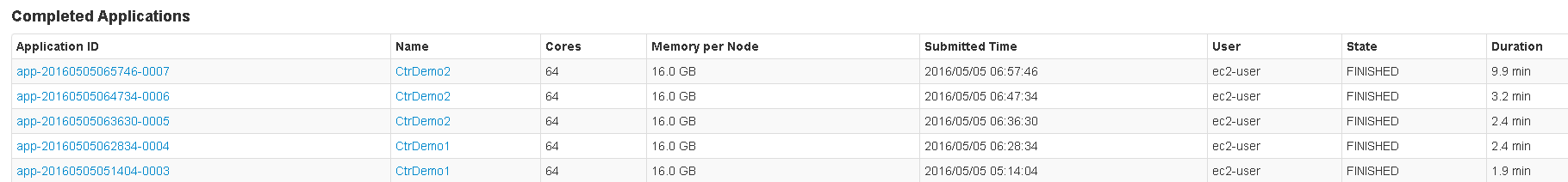
It takes about 2 minutes for the application to complete and output the following:

1
Area under ROC = 0.5177127622153417

We get AUROC slightly better than a random guess (AUROC = 0.5), which is not so bad for our first approach, but we can definitely do better.

Experimenting with more features

Let’s try to select more features and see how it affects our metrics.

For this we created a new version of our app CtrDemo2 where we can easily select features we want to include. We use VectorAssembler to assemble multiple feature vectors into a single features one:

1
2
3
4
val assembledDf = new VectorAssembler()
  .setInputCols(categoricalColumnsVectors.toArray)
  .setOutputCol("features")
  .transform(encodedDf)

The results are the following:

  • with additionally included device_type: AUROC = 0.531015564807053
  • + time_day and time_hour: AUROC = 0.5555488992624483
  • + C15, C16, C17, C18, C19, C20, C21: AUROC = 0.7000630113145946

You can notice how the AUROC is being improved as we add more and more features. This comes with the cost of the training time:

We didn’t include high-cardinality features such as device_ip and device_id as they will blow up the feature vector size. One may consider applying techniques such as feature hashing to reduce the dimension. We will leave it out of this blog post’s scope.

Tuning algorithm parameters

Tuning algorithm parameters is a search problem. We will use Spark Pipeline API with a Grid Search technique. Grid search evaluates a model for each combination of algorithm parameters specified in a grid (do not confuse with data grid).

Pipeline API supports model selection using cross-validation technique. For each set of parameters it trains the given Estimator and evaluates it using the given Evaluator. We will use BinaryClassificationEvaluator that has AUROC as a metric by default.

1
2
3
4
5
6
7
8
9
10
11
12
13
14
15
16
val lr = new LogisticRegression().setLabelCol("click")
val pipeline = new Pipeline().setStages(Array(assembler, lr))

val paramGrid = new ParamGridBuilder()
  .addGrid(lr.regParam, Array(0.01 , 0.1 /*, 1.0 */))
  .addGrid(lr.elasticNetParam, Array(0.0 /*, 0.5 , 1.0 */))
  .addGrid(lr.fitIntercept, Array(false /*, true */))
  .build()

val cv = new CrossValidator()
  .setEstimator(pipeline)
  .setEvaluator(new BinaryClassificationEvaluator().setLabelCol("click"))
  .setEstimatorParamMaps(paramGrid)
  .setNumFolds(3)

val cvModel = cv.fit(encodedTrainDf)

We included two regularization parameters 0.01 and 0.1 in our search grid for now, others are commented out for now.

Output the best set of parameters:

1
2
3
4
5
6
7
println("Grid search results:")
cvModel.getEstimatorParamMaps.zip(cvModel.avgMetrics).foreach(println)

println("Best set of parameters found:" + cvModel.getEstimatorParamMaps
  .zip(cvModel.avgMetrics)
  .maxBy(_._2)
  ._1)

Use the best model to predict test dataset loaded from the data grid:

1
2
3
val predictionDf = cvModel.transform(encodedTestDf).select("id", "probability").map {
  case Row(id: String, probability: Vector) => (id, probability(1))
}.toDF("id", "click")

Then the results are saved back to csv on hdfs, so we can submit them to Kaggle, see the complete listing in CtrDemo3.

It takes about 27 mins to train and compare models for two regularization parameters 0.01 and 0.1. The results are:

1
2
3
4
5
6
7
8
9
10
11
12
13
14
15
16
17
Grid search results:
({
	logreg_2b70e3edf1f0-elasticNetParam: 0.0,
	logreg_2b70e3edf1f0-fitIntercept: false,
	logreg_2b70e3edf1f0-regParam: 0.01
},0.7000655195682837)
({
	logreg_2b70e3edf1f0-elasticNetParam: 0.0,
	logreg_2b70e3edf1f0-fitIntercept: false,
	logreg_2b70e3edf1f0-regParam: 0.1
},0.697680175815199)

Best params found:{
	logreg_2b70e3edf1f0-elasticNetParam: 0.0,
	logreg_2b70e3edf1f0-fitIntercept: false,
	logreg_2b70e3edf1f0-regParam: 0.01
}

This simple logistic regression model has a rank of 1109 out of 1603 competitors in Kaggle.

The future improvements are only limited by data science skills and creativity. One may consider:

  • implement Logarithmic Loss function as an Evaluator since it’s used by Kaggle to calculate the model score. In our example we used AUROC
  • include other features that we didn’t select
  • generate additional features such click history of a user
  • use a hashing trick to reduce the features vector dimension
  • try other machine learning algorithms, the winner of competition used Field-aware Factorization Machines

Architecture

The following diagram demonstrates the design of machine learning application with InsightEdge.

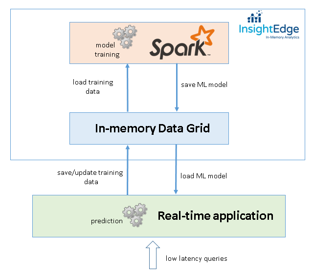
The key design advantages are:

  • the single platform converges analytical processing (machine learning) powered by Spark with transactional processing powered by custom real-time applications;
  • real-time applications can execute any OLTP query (read, insert, update, delete) on training data that is immediately available for Spark analytical queries or machine learning routines. There is no need to build a complex ETL pipeline that extracts training data from OLTP database with Kafka/Flume/HDFS. Besides the complexity, an ETL pipeline introduces unwanted latency that can be a stopper for reactive machine learning apps. With InsightEdge, Spark applications can view the live data;
  • the training data lives in the memory of data grid, which acts as an extension of Spark memory. This way we can load the data quicker;
  • An in-memory data grid is a general-purpose highly available and fault tolerant storage. With support of ACID transactions and SQL queries it becomes the primary storage for the application;
  • InsightEdge stack is scalable in both computation (Spark) and storage (data grid) tiers. This makes it attractive for large-scale machine learning.

Summary

In this blog post we demonstrated how to use machine learning algorithms with InsightEdge. We went through typical stages:

  • interactive data exploration with Zeppelin
  • feature selection and transformation
  • training predictive models
  • calculating model metrics
  • tuning parameters

We didn’t have a goal to build a perfect predictive model, so there is great room for improvement.

In the architecture section we discussed how the typical design may look like, what are the benefits of using InsightEdge for machine learning.

The Zeppelin notebook can be found here and submittable spark apps here

Comments